

除了整合差异相对较小的scRNA-seq数据集外,liger也能用于整合数据差异较大、甚至研究的对象完全不同的多组学。本文将以scRNA-seq和scATAC-seq为例,展示liger多组学整合的相关流程。scRNA-seq描述了细胞的转录组特征,而scATAC-seq则描述了细胞基因组开放性的特征,显然这两种组学特征之间存在着某种相关性,大胆一点我们可以认为整体上呈现正相关。通过scRNA-seq和scATAT-seq的整合分析,我们不光能够更加全面地描述细胞的特征,也能从开放性和RNA的角度上去推测可能的基因表达调控模式。尽管现在已经有了一些多组学测序的技术,例如10x的Single Cell Multiome ATAC Gene Expression,但更多的组学特征以及技术上仍有待进一步的突破,因此liger依然给我们提供了一个非常好的窗口帮助我们理解单细胞的生命特征。
对不同的数据集进行整合,数据集之间需要有一些共有的对象来作为feature,并且这些feature在不同的数据集之间应当存在着某种整体上的相关性(例如某一个基因越开放,则通常它的表达量就越高;某一个基因body上非CpG甲基化程度越高,则该基因通常就越处于沉默状态)。对于ATAC-seq等表观组的数据,我们通常使用peak来表征其在某一个位点上的强弱。尽管我们也可以统计各个基因上的peak数量来作为ATAC-seq的表达矩阵,但liger的作者认为这么做的效果可能并不理想,原因有以下三点。
- Call peak通常是用全部细胞来做的,而这种方式很容易埋没一些稀有细胞群的信号。
- 基因body上的开放性往往是比较弥散的,不像一些调控元件可以call出非常明显的peak,因此peaking calling的算法可能会丢失大量的信息。
- Peak本身就类似于显著差异的变化,因此大量的信息被丢失,本身稀疏的数据变得更加稀疏。
Liger作者发现,使用scATAC-seq在基因body和promoter上的reads数就能很容易地表征某个基因的整体开放性水平,promoter区域可以选择TSS上下游2kb的区域。本文的分析使用10x提供的公共测试数据,并使用10x提供的cellranger和cellranger-atac进行比对。scRNA-seq数据为健康供体的10k PBMC数据,scATAC-seq数据也是健康供体的10k PBMC数据。scATAC-seq比对所用的reference来自直接从10x官网上下载的现成的GRCh38参考基因组与注释,该reference所用的基因组注释文件为GENCODE的第28版GRCh38基因组注释,下载该注释文件后我们手工构建一个scRNA-seq的reference,从而最大程度地保证了scRNA-seq和scATAC-seq所用的注释文件的一致性。
############################################
## Project: Liger-learning
## Script Purpose: joint analysis of scRNA-seq and chromatin accessibility
## Data: 2020.10.24
## Author: Yiming Sun
############################################

#sleep
ii <- 1
while(1){
  cat(paste("round",ii),sep = "n")
  ii <- ii 1
  Sys.sleep(30)
}

# general setting
setwd('/data/User/sunym/project/liger_learning/')
# library
library(Seurat)
library(ggplot2)
library(dplyr)
library(scibet)
library(Matrix)
library(tidyverse)
library(cowplot)
library(viridis)
library(pheatmap)
library(ComplexHeatmap)
library(networkD3)
library(liger)
library(parallel)
#my function
MySuggestLambda <- function(object,lambda,k,knn_k = 20,thresh = 1e-04,max.iters = 100,k2 = 500,ref_dataset = NULL,resolution = 1,parl_num){
  res <- matrix(ncol = 2,nrow = length(lambda))
  colnames(res) <- c('lambda','alignment')
  res[,'lambda'] <- lambda
  cl <- makeCluster(parl_num)
  clusterExport(cl,c('object','k','knn_k','thresh','max.iters','k2','ref_dataset','resolution'),envir = environment())
  clusterExport(cl,c('optimizeALS','quantileAlignSNF','calcAlignment'),envir = .GlobalEnv)
  alignment_score <- parLapply(cl = cl,lambda,function(x){
    object <- optimizeALS(object,k = k,lambda = x,thresh = thresh,max.iters = max.iters)
    object <- quantileAlignSNF(object,knn_k = knn_k,k2 = k2,ref_dataset = ref_dataset,resolution = resolution)
    return(calcAlignment(object))
  })
  stopCluster(cl)
  res[,'alignment'] <- (alignment_score %>% unlist())
  res <- as.data.frame(res)
  res[,1] <- as.numeric(as.character(res[,1]))
  res[,2] <- as.numeric(as.character(res[,2]))
  p <- ggplot(res,aes(x = lambda,y = alignment)) geom_point() geom_line()
  return(list(res,p))
}
scATAC-seq 数据准备
首先我们需要把GENCODE提供的gtf格式的基因组注释文件转换成bed格式的注释文件,再用bedmap等工具去寻找我们测序所得到的reads与基因组上的注释有哪些overlap。gtf文件的前五行为该注释文件的相关信息,需要先去掉。
[[email protected] annotation]$ head -n 5 gencode.v28.annotation.gtf
##description: evidence-based annotation of the human genome (GRCh38), version 28 (Ensembl 92)
##provider: GENCODE
##contact: [email protected]
##format: gtf
##date: 2018-03-23
为了方便写成脚本,我就直接在R中调用system函数了,实际过程中我们也可以直接在linux终端进行操作。
# 1.joint analysis of scRNA-seq and chromatin accessibility
# pre-prapare scTATA data
#sort by chromosome start position and end position for fragment, gene and promoter
system('gunzip ./data/10k_pbmc/scATAC/fragments.tsv.gz')
system('tail -n 6 ./data/10k_pbmc/annotation/gencode.v28.annotation.gtf > ./data/10k_pbmc/annotation/genes_split.gtf')
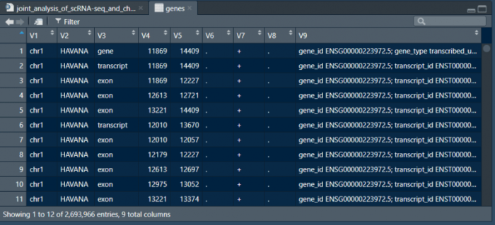
genes <- read.table('./data/10k_pbmc/annotation/genes_split.gtf',sep = 't')读入gtf文件后我们需要对条目进行筛选和整理。V1列表示所在的染色体,V4和V5分别表示了该片段在染色体上的起始位置,V7表示该片段位于正义链还是反义链,V9列则是对该片段名称的注释。我们筛选V3列为gene的条目,并对V9列进行整理。
genes <- genes[genes[,3] == 'gene',]
gene_name <- unlist(strsplit(as.character(genes[,9]),split = '; ',fixed = TRUE))
gene_name <- gene_name[grepl(pattern = 'gene_name',gene_name)]
gene_name <- sub(pattern = 'gene_name ',replacement = '',gene_name)
genes[,9] <- gene_name
genes <- genes[,c(1,4,5,9,6,7)]
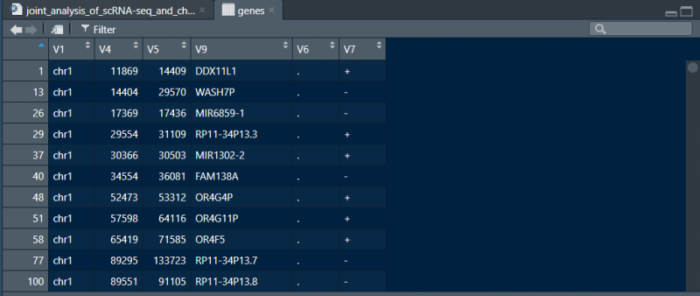
这样我们就得到了bed类似格式的注释文件。同理我们也可以利用TSS得到promoter的位置信息,不过需要注意正义链和反义链。构建好基因和promoter的两个表格后,将其保存为bed文件即可。
promoter <- as.data.frame(matrix(nrow = dim(genes)[1],ncol = dim(genes)[2]))
promoter[,c(1,4,5,6)] <- genes[,c(1,4,5,6)]
for (i in 1:dim(promoter)[1]) {
  if(promoter[i,6] == ' '){
    if ((as.numeric(genes[i,2])-2000) >= 0){
      promoter[i,2] <- as.numeric(genes[i,2])-2000
    }else{
      promoter[i,2] <- 0
    }
    promoter[i,3] <- as.numeric(genes[i,2]) 2000
  } else if(promoter[i,6] == '-'){
    if ((as.numeric(genes[i,3])-2000) >= 0){
      promoter[i,2] <- as.numeric(genes[i,3])-2000
    }else{
      promoter[i,2] <- 0
    }
    promoter[i,3] <- as.numeric(genes[i,3]) 2000
  }
}
write.table(genes,file = './data/10k_pbmc/annotation/genes.bed',sep = 't',col.names = FALSE,row.names = FALSE,quote = FALSE)
write.table(promoter,file = './data/10k_pbmc/annotation/promoter.bed',sep = 't',col.names = FALSE,row.names = FALSE,quote = FALSE)
在用bedmap做overlap之前需要先对reads和bed文件进行排序,按照染色体、起始位置、结束位置三者的先后顺序进行排序。排序完成后即可用bedmap计算overlap。
system('/data/User/sunym/software/BEDOPS/bin/sort-bed --max-mem 50G ./data/10k_pbmc/scATAC/fragments.tsv > ./data/10k_pbmc/scATAC/atac_fragments.sort.bed')
system('/data/User/sunym/software/BEDOPS/bin/sort-bed --max-mem 50G ./data/10k_pbmc/annotation/genes.bed > ./data/10k_pbmc/annotation/genes.sort.bed')
system('/data/User/sunym/software/BEDOPS/bin/sort-bed --max-mem 50G ./data/10k_pbmc/annotation/promoter.bed > ./data/10k_pbmc/annotation/promoters.sort.bed')
#Use bedmap command to calculate overlapping elements between indexes and fragment output files
system('/data/User/sunym/software/BEDOPS/bin/bedmap --ec --delim "t" --echo --echo-map-id ./data/10k_pbmc/annotation/promoters.sort.bed ./data/10k_pbmc/scATAC/atac_fragments.sort.bed > ./data/10k_pbmc/scATAC/atac_promoters_bc.bed')
system('/data/User/sunym/software/BEDOPS/bin/bedmap --ec --delim "t" --echo --echo-map-id ./data/10k_pbmc/annotation/genes.sort.bed ./data/10k_pbmc/scATAC/atac_fragments.sort.bed > ./data/10k_pbmc/scATAC/atac_genes_bc.bed')
构建liger对象
读入bedmap计算overlap后的输出文件。
#import the bedmap outputs into the R
genes.bc <- read.table(file = "./data/10k_pbmc/scATAC/atac_genes_bc.bed", sep = "t", as.is = c(4,7), header = FALSE)
promoters.bc <- read.table(file = "./data/10k_pbmc/scATAC/atac_promoters_bc.bed", sep = "t", as.is = c(4,7), header = FALSE)
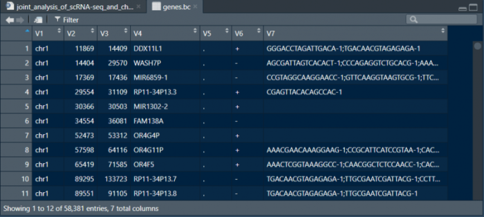
可以看到V7列包括了所有与该基因有overlap的细胞的barcode。筛选至少覆盖1500个基因的细胞为有效的细胞,并与peak数据中过滤得到的barcode做overlap,将这部分细胞用于后续的分析。
#load scATAC peak filted barcode data
barcodes <- read.table(file = './data/10k_pbmc/scATAC/filtered_peak_bc_matrix/barcodes.tsv',sep = 't',as.is = TRUE,header = FALSE)$V1
#filter the barcode with bad quality
bc <- genes.bc[,7]
bc_split <- strsplit(bc,";")
bc_split_vec <- unlist(bc_split)
bc_counts <- table(bc_split_vec)
bc_filt <- names(bc_counts)[bc_counts > 1500]
barcodes <- intersect(bc_filt,barcodes)
使用liger自带的makeFeatureMatrix函数对bedmap的输出结果进行处理,得到单个细胞在各个基因及其promoter上的reads数的表达矩阵,用该矩阵和scRNA-seq表达矩阵构建liger对象。
#use LIGER's makeFeatureMatrix function to calculate accessibility counts for gene body and promoter
gene.counts <- makeFeatureMatrix(genes.bc, barcodes)
promoter.counts <- makeFeatureMatrix(promoters.bc, barcodes)
gene.counts <- gene.counts[order(rownames(gene.counts)),]
promoter.counts <- promoter.counts[order(rownames(promoter.counts)),]
PBMCs <- gene.counts   promoter.counts
colnames(PBMCs)=paste0("PBMC_",colnames(PBMCs))
#load scRNA-seq data
PBMC.rna <- read10X(sample.dirs = './data/10k_pbmc/scRNA/filtered_feature_bc_matrix/',sample.names = 'rna')
#create a LIGER object
PBMC.data <- list(atac = PBMCs, rna = PBMC.rna)
int.PBMC <- createLiger(PBMC.data)
remove(list = ls()[ls() != 'int.PBMC'])
gc()
对liger对象进行标准化等一系列前期操作,注意只使用RNA-seq数据来挑选variable gene。
#normalize select gene and scale
int.PBMC <- normalize(int.PBMC)
int.PBMC <- selectGenes(int.PBMC, datasets.use = 2)
int.PBMC <- scaleNotCenter(int.PBMC)
非负矩阵分解
选择合适的参数K和λ进行矩阵分解。
#integrate NMF
#suggest lambda
suggestLambda(int.PBMC,lambda.test = seq(1,20,1),k = 25,num.cores = 10)
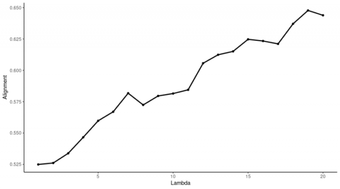
看这趋势似乎还在一路走高,一般建议λ的取值范围为0.25到60。经过后续的降维,我发现λ=10是个不错的选择。
#suggest k
suggestK(object = int.PBMC,k.test = seq(10,30,1),lambda = 10,num.cores = 10,plot.log2 = FALSE)
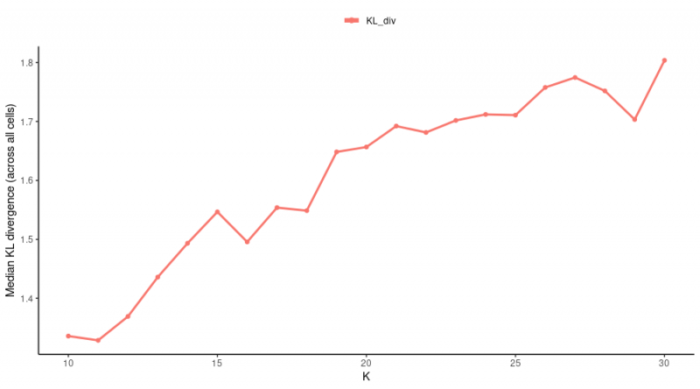
K在25左右就基本达到了饱和,因此我们选择K=25。根据我们后续的降维和聚类,这些值也都可以人为的进行调整,使得它尽可能地符合你的数据集,并让你的结果看起来“干净”。
#lambda = 10,k = 25
int.PBMC <- optimizeALS(int.PBMC,k = 25,lambda = 10,max.iters = 30,thresh = 1e-06)
#Quantile Normalization and Joint Clustering
int.PBMC <- quantile_norm(int.PBMC,knn_k = 20,quantiles = 50,min_cells = 20,do.center = FALSE,
                            max_sample = 1000,refine.knn = TRUE,eps = 0.9)
int.PBMC <- louvainCluster(int.PBMC, resolution = 0.4)
可以看下总共聚出了多少个cluster。
> table([email protected])

   0    1    2    3    4    5    6    7    8    9   10   11
3360 2552 2484 2074 1976 1683 1629 1004  897  778  776  416
  12   13   14   15   16   17
 398  391  316  304  154  108
可视化
- UMAP
#Visualization and Downstream Analysis
int.PBMC <- runUMAP(int.PBMC)
all.plots <- plotByDatasetAndCluster(int.PBMC, axis.labels = c('UMAP 1', 'UMAP 2'),return.plots = TRUE)
head(all.plots[[1]]$data)
pdf(file = './res/fig_201112/plot_by_dataset_and_cluster.pdf',width = 8,height = 4)
all.plots[[1]]   all.plots[[2]]
dev.off()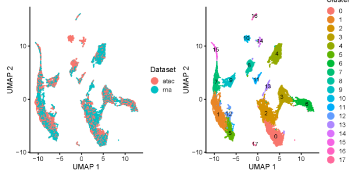
- 差异表达分析
#identify marker genes for each cluster
int.PBMC.wilcoxon <- runWilcoxon(int.PBMC, data.use = 'all', compare.method = 'clusters')
#filter the enriched gene yourself
int.PBMC.wilcoxon <- int.PBMC.wilcoxon[int.PBMC.wilcoxon$padj < 0.05,]
int.PBMC.wilcoxon <- int.PBMC.wilcoxon[int.PBMC.wilcoxon$logFC > 3,]
#top 20 markers of cluster 3 and 4
wilcoxon.cluster_3 <- int.PBMC.wilcoxon[int.PBMC.wilcoxon$group == 3, ]
wilcoxon.cluster_3 <- wilcoxon.cluster_3[order(wilcoxon.cluster_3$padj), ]
markers.cluster_3 <- wilcoxon.cluster_3[1:20, ]
wilcoxon.cluster_4 <- int.PBMC.wilcoxon[int.PBMC.wilcoxon$group == 4, ]
wilcoxon.cluster_4 <- wilcoxon.cluster_4[order(wilcoxon.cluster_4$padj), ]
markers.cluster_4 <- wilcoxon.cluster_4[1:20, ]
具体看下cluster_3和cluster_4中有哪些基因(RNA和开放性)被富集到。
> markers.cluster_3
          feature group   avgExpr    logFC statistic       auc pval padj pct_in pct_out
93440  AC092580.4     3 -16.77217 5.369608  27507364 0.6898446    0    0    100     100
96414        CCL5     3 -11.02601 9.269639  32396409 0.8124547    0    0    100     100
96562        CD8A     3 -13.57582 6.735737  29898397 0.7498083    0    0    100     100
97532        CST7     3 -12.67376 7.845358  31058233 0.7788952    0    0    100     100
98887        CTSW     3 -14.43134 6.331951  28632810 0.7180692    0    0    100     100
99965       EOMES     3 -16.80980 4.705106  26695598 0.6694867    0    0    100     100
101646       GZMA     3 -14.08326 7.198335  29369425 0.7365424    0    0    100     100
101649       GZMK     3 -14.48547 7.763756  30122792 0.7554357    0    0    100     100
101650       GZMM     3 -13.68788 6.104824  28699408 0.7197393    0    0    100     100
102068       HOPX     3 -15.09229 5.371568  27605779 0.6923127    0    0    100     100
102524       IL32     3 -11.36195 6.950100  29875540 0.7492350    0    0    100     100
103205      KLRB1     3 -14.85939 6.264977  28100056 0.7047085    0    0    100     100
103213      KLRG1     3 -11.01856 7.183600  31721918 0.7955395    0    0    100     100
103361       LAG3     3 -18.79355 3.451362  24980309 0.6264698    0    0    100     100
103916       LYAR     3 -12.56974 5.956998  29655544 0.7437179    0    0    100     100
104130       MATK     3 -15.48198 5.632058  28084886 0.7043280    0    0    100     100
105193       NCR3     3 -17.23250 4.670144  26521096 0.6651105    0    0    100     100
105421       NKG7     3 -11.84455 8.689092  31538326 0.7909353    0    0    100     100
107166       PRF1     3 -13.84797 7.254678  30034053 0.7532103    0    0    100     100
107282       PRR5     3 -12.95011 4.999333  28880551 0.7242821    0    0    100     100
> markers.cluster_4
        feature group    avgExpr     logFC statistic       auc pval padj pct_in pct_out
124628   ADAM28     4 -14.686500  6.687493  28617138 0.7494493    0    0    100     100
125560 ARHGAP24     4 -13.124318  5.737005  28321370 0.7417034    0    0    100     100
126016    BANK1     4  -9.488431  9.653939  34707167 0.9089400    0    0    100     100
126063   BCL11A     4 -11.083597  7.253749  31052386 0.8132255    0    0    100     100
126149      BLK     4 -13.199351  7.485614  30191285 0.7906743    0    0    100     100
126152     BLNK     4 -16.619583  4.727523  25910558 0.6785671    0    0    100     100
127204     CD22     4 -11.490107  9.400583  32656222 0.8552281    0    0    100     100
127206     CD24     4 -17.198765  5.403821  26269448 0.6879660    0    0    100     100
127229     CD37     4  -7.768716  6.736971  33587469 0.8796164    0    0    100     100
127236     CD40     4 -15.849347  5.536785  27024648 0.7077438    0    0    100     100
127244     CD52     4  -9.103628  5.641797  30316353 0.7939497    0    0    100     100
127257     CD74     4  -6.196057  6.340909  34263853 0.8973301    0    0    100     100
127258    CD79A     4  -8.407126 12.678446  35987290 0.9424649    0    0    100     100
127259    CD79B     4  -9.626859 11.530288  34664105 0.9078122    0    0    100     100
127313   CDCA7L     4 -16.539789  4.886703  26014286 0.6812836    0    0    100     100
127941   COBLL1     4 -16.594804  4.437667  25557096 0.6693103    0    0    100     100
130946  FAM129C     4 -13.668283  6.205986  28893095 0.7566762    0    0    100     100
131192      FAU     4  -8.118877  4.119389  29235631 0.7656468    0    0    100     100
131273    FCER2     4 -14.723589  6.953663  28740433 0.7526782    0    0    100     100
131280   FCGR2B     4 -19.050128  3.596260  23898797 0.6258814    0    0    100     100
>
cluster_3中富集到了CD8A,cluster_4中富集到了CD79A,感觉都是挺重要的基因,可以看下这两个基因的表达情况。
#feature plot on umap
# CD8A for cluster 2 and CD79A for cluster 4
CD8A <- plotGene(int.PBMC, "CD8A", axis.labels = c('UMAP 1', 'UMAP 2'), return.plots = TRUE)
CD79A <- plotGene(int.PBMC, "CD79A", axis.labels = c('UMAP 1', 'UMAP 2'), return.plots = TRUE)
pdf(file = './res/fig_201112/marker_for_cluster_3_and_4.pdf',width = 9,height = 6)
plot_grid(CD8A[[2]],CD79A[[2]],CD8A[[1]],CD79A[[1]], ncol=2)
dev.off()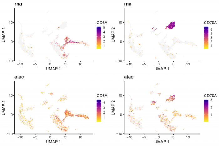
- metagene
也可以从metagene的角度去探究基因的差异表达。
#gene loading plot
# gene loading plot of factor12
all.plots <- plotGeneLoadings(int.PBMC, return.plots = TRUE,do.spec.plot = FALSE)
pdf(file = './res/fig_201112/gene_loading_factor_18.pdf')
all.plots[[18]]
dev.off()
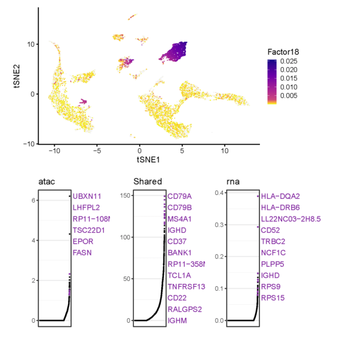
可以看到metagene_18在cluster_4中特异性地高loading,两个数据集中CD79A和CD79B都对metagene_18有很高的贡献,这与我们之前找到的差异表达基因相吻合。可以继续来看下不同数据集各自对metagene_18的贡献,如何导出gene loading plot背后的数据可以参考文章使用liger整合单细胞RNA-seq数据集。
# feature plot
TCL1A <- plotGene(int.PBMC, "TCL1A", axis.labels = c('UMAP 1', 'UMAP 2'), return.plots = TRUE)
RPS9 <- plotGene(int.PBMC, "RPS9", axis.labels = c('UMAP 1', 'UMAP 2'), return.plots = TRUE)
pdf(file = './res/fig_201112/RPS9_TCL1A_plot_for_RNA_and_ATAC.pdf',width = 9,height = 6)
plot_grid(RPS9[[2]],TCL1A[[2]],RPS9[[1]],TCL1A[[1]], ncol=2)
dev.off()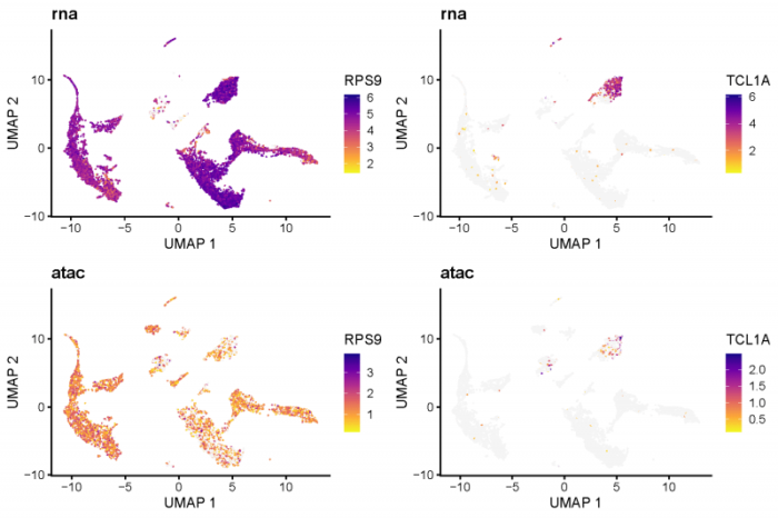
可以看到RPS9作为一种核糖体蛋白在各种细胞中均有表达,而在分泌抗体的B细胞中这种表达显然会更高,这与RNA-seq的表达谱相一致。不过在ATAC-seq的表达谱中,B细胞中的RPS9的开放性似乎并不是最高的,说明控制RPS9转录的机制可能不止基因组的开放性这一种。TCL1A的转录组和ATAC-seq谱在都在B细胞中高表达,显示出了开放性与基因表达的整体正相关。
- Pseudo peak
这也是liger非常有意思的一点,即它可以利用一个数据集的特征去预测另一个数据集的特征。想法也非常简单,数据集1中的细胞A周围有k个数据集2中的细胞,那么A的特征应该和这k个细胞很像,利用简单的平均我们就可以预测出A中数据集2特有的特征。在本例中,ATAC-seq的peak是数据集2(ATAC-seq数据集)特有的特征,那么我可以利用liger预测出数据集1(RNA-seq数据集)中细胞的peak特征,就像我们同时对一个细胞测定了RNA和ATAC一样,尽管这种ATAC是预测出来的。
首先我们需要先读入ATAC-seq的peak的数据,并对barcode进行过滤,使得它完全包含于我们之前使用reads构建的ATAC-seq表达谱中。
# Pseudo single multi-omic data (scRNA-seq and scATAC-seq)
#load scATAC peak data
barcodes <- read.table(file = './data/10k_pbmc/scATAC/filtered_peak_bc_matrix/barcodes.tsv',sep = 't',as.is = TRUE,header = FALSE)$V1
barcodes <- paste('PBMC',barcodes,sep = '_')
peak.names <- read.table(file = './data/10k_pbmc/scATAC/filtered_peak_bc_matrix/peaks.bed', sep = 't', header = FALSE)
peak.names <- paste0(peak.names$V1, ':', peak.names$V2, '-', peak.names$V3)
pmat <- readMM(file = './data/10k_pbmc/scATAC/filtered_peak_bc_matrix/matrix.mtx')
colnames(pmat) <- barcodes
rownames(pmat) <- peak.names
pmat <- pmat[,colnames([email protected]$atac)]
peak的个数还是相当多的,为了简化我们的运算量,我们需要从中挑选出不同的cluster之间差异表达的peak。
> dim(pmat)
[1] 94534  9642
虽然liger的官方教程说可以直接把pmat赋值给ATAC的表达矩阵,然后只用ATAC做差异表达分析即可,但我跑的时候又是各种奇怪的报错,所以变通一下,我们用seurat来构建ATAC的表达矩阵然后来做差异表达分析。
#cell-type-specific accessibility
#create seurat for pmat
pmat_seurat <- CreateSeuratObject(counts = pmat,project = 'pmat')
pmat_seurat <- NormalizeData(pmat_seurat, normalization.method = "LogNormalize", scale.factor = 10000)
pmat_seurat <- ScaleData(pmat_seurat, features = rownames(pmat_seurat))
cell_type <- [email protected]
cell_type <- cell_type[colnames(pmat_seurat)]
pmat_seurat$cell_type <- cell_type
table(pmat_seurat$cell_type)
Idents(pmat_seurat) <- 'cell_type'
#find the DEPeak across the cluster
pmat_marker <- FindAllMarkers(pmat_seurat, only.pos = TRUE, logfc.threshold = 0.25)
pmat_marker <- pmat_marker[pmat_marker$p_val_adj < 0.05,]
peaks.sel <- unique(pmat_marker$gene)
peaks.sel就是我们挑选出的在cluster之间差异表达的peak。我们用这组peak来过滤pmat(用于预测RNA-seq中的peak)以及pmat_seurat(用于画图)。
#filter the pmat seurat object and scale the express
pmat_seurat <- pmat_seurat[peaks.sel,]
pmat_seurat <- NormalizeData(pmat_seurat, normalization.method = "LogNormalize", scale.factor = 10000)
pmat_seurat <- ScaleData(pmat_seurat, features = rownames(pmat_seurat),do.center = FALSE)
#filter the pmat object to impute the RNA-seq cell's ATAC peaks
pmat <- pmat[peaks.sel,]
int.PBMC.ds <- int.PBMC
[email protected][['atac']] <- pmat
int.PBMC.ds <- normalize(int.PBMC.ds)
使用ATAC-seq数据预测RNA-seq数据中的peak。
#predict the accessibility profile for scRNA-seq data
int.PBMC.ds <- imputeKNN(int.PBMC.ds, reference = 'atac',queries = 'rna',knn_k = 20,norm = TRUE,scale = FALSE)
预测后的数据就覆盖了原来的RNA-seq的表达谱。
> [email protected]$rna[1:3,1:3]
3 x 3 sparse Matrix of class "dgCMatrix"
                         rna_AAACCCAAGCGCCCAT rna_AAACCCAAGGTTCCGC
chr6:111086981-111088830         .                    0.0001584052
chr17:82126355-82127872          0.0007113352         .
chr8:19496551-19497709           .                    .
                         rna_AAACCCACAGACAAGC
chr6:111086981-111088830         4.491621e-05
chr17:82126355-82127872          2.747334e-04
chr8:19496551-19497709           1.823305e-04
现在我们就得到了单细胞RNA-seq数据集中细胞的转录组和(预测的)peak的特征,我们就可以去寻找基因表达与开放性元件的调控关系。想法也非常简单,我们可以计算一个基因的表达量与其上下游500kb范围内的peak强度的相关性。如果你希望扩大或者缩小这个上下游的范围,你可以用我修改过后的函数,peak_range以一个碱基为单位。
MyLinkGenesAndPeaks <- function(gene_counts, peak_counts, genes.list = NULL, dist = "spearman",
                                                     alpha = 0.05, path_to_coords, peak_range) {
  ## check dependency
  if (!requireNamespace("GenomicRanges", quietly = TRUE)) {
    stop("Package "GenomicRanges" needed for this function to work. Please install it by command:n",
         "BiocManager::install('GenomicRanges')",
         call. = FALSE
    )
  }

  if (!requireNamespace("IRanges", quietly = TRUE)) {
    stop("Package "IRanges" needed for this function to work. Please install it by command:n",
         "BiocManager::install('IRanges')",
         call. = FALSE
    )
  }

  ### make Granges object for peaks
  peak.names <- strsplit(rownames(peak_counts), "[:-]")
  chrs <- Reduce(append, lapply(peak.names, function(peak) {
    peak[1]
  }))
  chrs.start <- Reduce(append, lapply(peak.names, function(peak) {
    peak[2]
  }))
  chrs.end <- Reduce(append, lapply(peak.names, function(peak) {
    peak[3]
  }))
  peaks.pos <- GenomicRanges::GRanges(
    seqnames = chrs,
    ranges = IRanges::IRanges(as.numeric(chrs.start), end = as.numeric(chrs.end))
  )

  ### make Granges object for genes
  gene.names <- read.csv2(path_to_coords, sep = "t", header = FALSE, stringsAsFactors = F)
  gene.names <- gene.names[complete.cases(gene.names), ]
  genes.coords <- GenomicRanges::GRanges(
    seqnames = gene.names$V1,
    ranges = IRanges::IRanges(as.numeric(gene.names$V2), end = as.numeric(gene.names$V3))
  )
  names(genes.coords) <- gene.names$V4

  ### construct regnet
  gene_counts <- t(gene_counts) # cell x genes
  peak_counts <- t(peak_counts) # cell x genes

  # find overlap peaks for each gene
  if (missing(genes.list)) {
    genes.list <- colnames(gene_counts)
  }
  missing_genes <- !genes.list %in% names(genes.coords)
  if (sum(missing_genes)!=0){
    print(
      paste0(
        "Removing ", sum(missing_genes),
        " genes not found in given gene coordinates..."
      )
    )
  }
  genes.list <- genes.list[!missing_genes]
  genes.coords <- genes.coords[genes.list]

  print("Calculating correlation for gene-peak pairs...")
  each.len <- 0
  # assign('each.len', 0, envir = globalenv())

  elements <- lapply(seq(length(genes.list)), function(pos) {
    gene.use <- genes.list[pos]
    # re-scale the window for each gene
    gene.loci <- GenomicRanges::trim(suppressWarnings(GenomicRanges::promoters(GenomicRanges::resize(
      genes.coords[gene.use],
      width = 1, fix = "start"
    ),
    upstream = peak_range, downstream = peak_range
    )))
    peaks.use <- S4Vectors::queryHits(GenomicRanges::findOverlaps(peaks.pos, gene.loci))
    if ((x <- length(peaks.use)) == 0L) { # if no peaks in window, skip this iteration
      return(list(NULL, as.numeric(each.len), NULL))
    }
    ### compute correlation and p-adj for genes and peaks ###
    res <- suppressWarnings(psych::corr.test(
      x = gene_counts[, gene.use], y = as.matrix(peak_counts[, peaks.use]),
      method = dist, adjust = "holm", ci = FALSE, use = "complete"
    ))
    pick <- res[["p"]] < alpha # filter by p-value
    pick[is.na(pick)] <- FALSE

    if (sum(pick) == 0) { # if no peaks are important, skip this iteration
      return(list(NULL, as.numeric(each.len), NULL))
    }
    else {
      res.corr <- as.numeric(res[["r"]][pick])
      peaks.use <- peaks.use[pick]
    }
    # each.len <<- each.len   length(peaks.use)
    assign('each.len', each.len   length(peaks.use), envir = parent.frame(2))
    return(list(as.numeric(peaks.use), as.numeric(each.len), res.corr))
  })

  i_index <- Reduce(append, lapply(elements, function(ele) {
    ele[[1]]
  }))
  p_index <- c(0, Reduce(append, lapply(elements, function(ele) {
    ele[[2]]
  })))
  value_list <- Reduce(append, lapply(elements, function(ele) {
    ele[[3]]
  }))

  # make final sparse matrix
  regnet <- sparseMatrix(
    i = i_index, p = p_index, x = value_list,
    dims = c(ncol(peak_counts), length(genes.list)),
    dimnames = list(colnames(peak_counts), genes.list)
  )

  return(regnet)
}
这个相关性的计算还挺漫长的,可以先去吃个饭2333。
#find peaks and genes strongly corrected
gmat = [email protected][['rna']]
pseudo_pmat = [email protected][['rna']]
regnet = MyLinkGenesAndPeaks(gene_counts = gmat, peak_counts = pseudo_pmat, dist = 'spearman', alpha = 0.05, path_to_coords = './data/10k_pbmc/annotation/genes.bed',peak_range = 500000)
对于我们关注的基因TCL1A,我们可以来看下有没有与其表达量高相关的peak。
> which(regnet[,'TCL1A'] > 0.6)
chr14:95456861-95457458
                    963
> saveRDS(regnet,file = './res/fig_201112/regnet.rds')
我们成功找到了一个高相关的peak,相关性系数为0.73。为了进一步验证我们方法的可靠性,我们可以画出原始的peak的强度和RNA-seq的表达量。
#convert to seurat and plot
tsne.obj <- CreateDimReducObject(embeddings = [email protected][colnames(pmat_seurat),], key = "UMAP_",global = TRUE)
pmat_seurat[['tsne']] <- tsne.obj
TCL1A <- plotGene(int.PBMC, "TCL1A", axis.labels = c('UMAP_1', 'UMAP_2'), return.plots = TRUE)
peak1 <- FeaturePlot(pmat_seurat,features = 'chr14:95456861-95457458',reduction = 'tsne')
pdf(file = './res/fig_201112/high_related_peak_gene_dimplot.pdf',width = 9,height = 9)
peak1[[1]] / TCL1A[[2]]
dev.off()
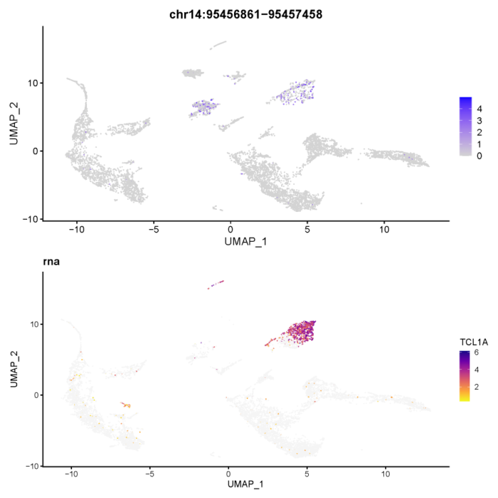
确实在B细胞群中,RNA的表达和peak的强度呈现明显的正相关,同时我们也注意到另一群细胞中peak的强度很高,但RNA的表达量却几乎没有,这其中的基因表达调控机制或许也值得我们后续的研究和探讨。
完整代码
############################################
## Project: Liger-learning
## Script Purpose: joint analysis of scRNA-seq and chromatin accessibility
## Data: 2020.10.24
## Author: Yiming Sun
############################################

#sleep
ii <- 1
while(1){
  cat(paste("round",ii),sep = "n")
  ii <- ii 1
  Sys.sleep(30)
}

# general setting
setwd('/data/User/sunym/project/liger_learning/')
# library
library(Seurat)
library(ggplot2)
library(dplyr)
library(scibet)
library(Matrix)
library(tidyverse)
library(cowplot)
library(viridis)
library(pheatmap)
library(ComplexHeatmap)
library(networkD3)
library(liger)
library(parallel)
#my function
MySuggestLambda <- function(object,lambda,k,knn_k = 20,thresh = 1e-04,max.iters = 100,k2 = 500,ref_dataset = NULL,resolution = 1,parl_num){
  res <- matrix(ncol = 2,nrow = length(lambda))
  colnames(res) <- c('lambda','alignment')
  res[,'lambda'] <- lambda
  cl <- makeCluster(parl_num)
  clusterExport(cl,c('object','k','knn_k','thresh','max.iters','k2','ref_dataset','resolution'),envir = environment())
  clusterExport(cl,c('optimizeALS','quantileAlignSNF','calcAlignment'),envir = .GlobalEnv)
  alignment_score <- parLapply(cl = cl,lambda,function(x){
    object <- optimizeALS(object,k = k,lambda = x,thresh = thresh,max.iters = max.iters)
    object <- quantileAlignSNF(object,knn_k = knn_k,k2 = k2,ref_dataset = ref_dataset,resolution = resolution)
    return(calcAlignment(object))
  })
  stopCluster(cl)
  res[,'alignment'] <- (alignment_score %>% unlist())
  res <- as.data.frame(res)
  res[,1] <- as.numeric(as.character(res[,1]))
  res[,2] <- as.numeric(as.character(res[,2]))
  p <- ggplot(res,aes(x = lambda,y = alignment)) geom_point() geom_line()
  return(list(res,p))
}

MyLinkGenesAndPeaks <- function(gene_counts, peak_counts, genes.list = NULL, dist = "spearman",
                                alpha = 0.05, path_to_coords, peak_range) {
  ## check dependency
  if (!requireNamespace("GenomicRanges", quietly = TRUE)) {
    stop("Package "GenomicRanges" needed for this function to work. Please install it by command:n",
         "BiocManager::install('GenomicRanges')",
         call. = FALSE
    )
  }

  if (!requireNamespace("IRanges", quietly = TRUE)) {
    stop("Package "IRanges" needed for this function to work. Please install it by command:n",
         "BiocManager::install('IRanges')",
         call. = FALSE
    )
  }

  ### make Granges object for peaks
  peak.names <- strsplit(rownames(peak_counts), "[:-]")
  chrs <- Reduce(append, lapply(peak.names, function(peak) {
    peak[1]
  }))
  chrs.start <- Reduce(append, lapply(peak.names, function(peak) {
    peak[2]
  }))
  chrs.end <- Reduce(append, lapply(peak.names, function(peak) {
    peak[3]
  }))
  peaks.pos <- GenomicRanges::GRanges(
    seqnames = chrs,
    ranges = IRanges::IRanges(as.numeric(chrs.start), end = as.numeric(chrs.end))
  )

  ### make Granges object for genes
  gene.names <- read.csv2(path_to_coords, sep = "t", header = FALSE, stringsAsFactors = F)
  gene.names <- gene.names[complete.cases(gene.names), ]
  genes.coords <- GenomicRanges::GRanges(
    seqnames = gene.names$V1,
    ranges = IRanges::IRanges(as.numeric(gene.names$V2), end = as.numeric(gene.names$V3))
  )
  names(genes.coords) <- gene.names$V4

  ### construct regnet
  gene_counts <- t(gene_counts) # cell x genes
  peak_counts <- t(peak_counts) # cell x genes

  # find overlap peaks for each gene
  if (missing(genes.list)) {
    genes.list <- colnames(gene_counts)
  }
  missing_genes <- !genes.list %in% names(genes.coords)
  if (sum(missing_genes)!=0){
    print(
      paste0(
        "Removing ", sum(missing_genes),
        " genes not found in given gene coordinates..."
      )
    )
  }
  genes.list <- genes.list[!missing_genes]
  genes.coords <- genes.coords[genes.list]

  print("Calculating correlation for gene-peak pairs...")
  each.len <- 0
  # assign('each.len', 0, envir = globalenv())

  elements <- lapply(seq(length(genes.list)), function(pos) {
    gene.use <- genes.list[pos]
    # re-scale the window for each gene
    gene.loci <- GenomicRanges::trim(suppressWarnings(GenomicRanges::promoters(GenomicRanges::resize(
      genes.coords[gene.use],
      width = 1, fix = "start"
    ),
    upstream = peak_range, downstream = peak_range
    )))
    peaks.use <- S4Vectors::queryHits(GenomicRanges::findOverlaps(peaks.pos, gene.loci))
    if ((x <- length(peaks.use)) == 0L) { # if no peaks in window, skip this iteration
      return(list(NULL, as.numeric(each.len), NULL))
    }
    ### compute correlation and p-adj for genes and peaks ###
    res <- suppressWarnings(psych::corr.test(
      x = gene_counts[, gene.use], y = as.matrix(peak_counts[, peaks.use]),
      method = dist, adjust = "holm", ci = FALSE, use = "complete"
    ))
    pick <- res[["p"]] < alpha # filter by p-value
    pick[is.na(pick)] <- FALSE

    if (sum(pick) == 0) { # if no peaks are important, skip this iteration
      return(list(NULL, as.numeric(each.len), NULL))
    }
    else {
      res.corr <- as.numeric(res[["r"]][pick])
      peaks.use <- peaks.use[pick]
    }
    # each.len <<- each.len   length(peaks.use)
    assign('each.len', each.len   length(peaks.use), envir = parent.frame(2))
    return(list(as.numeric(peaks.use), as.numeric(each.len), res.corr))
  })

  i_index <- Reduce(append, lapply(elements, function(ele) {
    ele[[1]]
  }))
  p_index <- c(0, Reduce(append, lapply(elements, function(ele) {
    ele[[2]]
  })))
  value_list <- Reduce(append, lapply(elements, function(ele) {
    ele[[3]]
  }))

  # make final sparse matrix
  regnet <- sparseMatrix(
    i = i_index, p = p_index, x = value_list,
    dims = c(ncol(peak_counts), length(genes.list)),
    dimnames = list(colnames(peak_counts), genes.list)
  )

  return(regnet)
}
# 1.joint analysis of scRNA-seq and chromatin accessibility
# pre-prapare scTATA data
#sort by chromosome start position and end position for fragment, gene and promoter
system('gunzip ./data/10k_pbmc/scATAC/fragments.tsv.gz')
system('tail -n  6 ./data/10k_pbmc/annotation/gencode.v28.annotation.gtf > ./data/10k_pbmc/annotation/genes_split.gtf')
genes <- read.table('./data/10k_pbmc/annotation/genes_split.gtf',sep = 't')
genes <- genes[genes[,3] == 'gene',]
gene_name <- unlist(strsplit(as.character(genes[,9]),split = '; ',fixed = TRUE))
gene_name <- gene_name[grepl(pattern = 'gene_name',gene_name)]
gene_name <- sub(pattern = 'gene_name ',replacement = '',gene_name)
genes[,9] <- gene_name
genes <- genes[,c(1,4,5,9,6,7)]
promoter <- as.data.frame(matrix(nrow = dim(genes)[1],ncol = dim(genes)[2]))
promoter[,c(1,4,5,6)] <- genes[,c(1,4,5,6)]
for (i in 1:dim(promoter)[1]) {
  if(promoter[i,6] == ' '){
    if ((as.numeric(genes[i,2])-2000) >= 0){
      promoter[i,2] <- as.numeric(genes[i,2])-2000
    }else{
      promoter[i,2] <- 0
    }
    promoter[i,3] <- as.numeric(genes[i,2]) 2000
  } else if(promoter[i,6] == '-'){
    if ((as.numeric(genes[i,3])-2000) >= 0){
      promoter[i,2] <- as.numeric(genes[i,3])-2000
    }else{
      promoter[i,2] <- 0
    }
    promoter[i,3] <- as.numeric(genes[i,3]) 2000
  }
}
write.table(genes,file = './data/10k_pbmc/annotation/genes.bed',sep = 't',col.names = FALSE,row.names = FALSE,quote = FALSE)
write.table(promoter,file = './data/10k_pbmc/annotation/promoter.bed',sep = 't',col.names = FALSE,row.names = FALSE,quote = FALSE)
system('/data/User/sunym/software/BEDOPS/bin/sort-bed --max-mem 50G ./data/10k_pbmc/scATAC/fragments.tsv > ./data/10k_pbmc/scATAC/atac_fragments.sort.bed')
system('/data/User/sunym/software/BEDOPS/bin/sort-bed --max-mem 50G ./data/10k_pbmc/annotation/genes.bed > ./data/10k_pbmc/annotation/genes.sort.bed')
system('/data/User/sunym/software/BEDOPS/bin/sort-bed --max-mem 50G ./data/10k_pbmc/annotation/promoter.bed > ./data/10k_pbmc/annotation/promoters.sort.bed')
#Use bedmap command to calculate overlapping elements between indexes and fragment output files
system('/data/User/sunym/software/BEDOPS/bin/bedmap --ec --delim "t" --echo --echo-map-id ./data/10k_pbmc/annotation/promoters.sort.bed ./data/10k_pbmc/scATAC/atac_fragments.sort.bed > ./data/10k_pbmc/scATAC/atac_promoters_bc.bed')
system('/data/User/sunym/software/BEDOPS/bin/bedmap --ec --delim "t" --echo --echo-map-id ./data/10k_pbmc/annotation/genes.sort.bed ./data/10k_pbmc/scATAC/atac_fragments.sort.bed > ./data/10k_pbmc/scATAC/atac_genes_bc.bed')


# load data
#load scATAC peak filted barcode data
barcodes <- read.table(file = './data/10k_pbmc/scATAC/filtered_peak_bc_matrix/barcodes.tsv',sep = 't',as.is = TRUE,header = FALSE)$V1
#import the bedmap outputs into the R
genes.bc <- read.table(file = "./data/10k_pbmc/scATAC/atac_genes_bc.bed", sep = "t", as.is = c(4,7), header = FALSE)
promoters.bc <- read.table(file = "./data/10k_pbmc/scATAC/atac_promoters_bc.bed", sep = "t", as.is = c(4,7), header = FALSE)
#filter the barcode with bad quality
bc <- genes.bc[,7]
bc_split <- strsplit(bc,";")
bc_split_vec <- unlist(bc_split)
bc_counts <- table(bc_split_vec)
bc_filt <- names(bc_counts)[bc_counts > 1500]
barcodes <- intersect(bc_filt,barcodes)
#use LIGER's makeFeatureMatrix function to calculate accessibility counts for gene body and promoter
gene.counts <- makeFeatureMatrix(genes.bc, barcodes)
promoter.counts <- makeFeatureMatrix(promoters.bc, barcodes)
gene.counts <- gene.counts[order(rownames(gene.counts)),]
promoter.counts <- promoter.counts[order(rownames(promoter.counts)),]
PBMCs <- gene.counts   promoter.counts
colnames(PBMCs)=paste0("PBMC_",colnames(PBMCs))
#load scRNA-seq data
PBMC.rna <- read10X(sample.dirs = './data/10k_pbmc/scRNA/filtered_feature_bc_matrix/',sample.names = 'rna')
#create a LIGER object
PBMC.data <- list(atac = PBMCs, rna = PBMC.rna)
int.PBMC <- createLiger(PBMC.data)
remove(list = ls()[ls() != 'int.PBMC'])
gc()
#normalize select gene and scale
int.PBMC <- normalize(int.PBMC)
int.PBMC <- selectGenes(int.PBMC, datasets.use = 2)
int.PBMC <- scaleNotCenter(int.PBMC)
#integrate NMF
#suggest lambda
suggestLambda(int.PBMC,lambda.test = seq(1,20,1),k = 25,num.cores = 10)
#suggest k
suggestK(object = int.PBMC,k.test = seq(10,30,1),lambda = 10,num.cores = 10,plot.log2 = FALSE)
#lambda = 10,k = 25
int.PBMC <- optimizeALS(int.PBMC,k = 25,lambda = 10,max.iters = 30,thresh = 1e-06)
#Quantile Normalization and Joint Clustering
int.PBMC <- quantile_norm(int.PBMC,knn_k = 20,quantiles = 50,min_cells = 20,do.center = FALSE,
                            max_sample = 1000,refine.knn = TRUE,eps = 0.9)
int.PBMC <- louvainCluster(int.PBMC, resolution = 0.4)
table([email protected])
#Visualization and Downstream Analysis
int.PBMC <- runUMAP(int.PBMC)
all.plots <- plotByDatasetAndCluster(int.PBMC, axis.labels = c('UMAP 1', 'UMAP 2'),return.plots = TRUE)
head(all.plots[[1]]$data)
pdf(file = './res/fig_201112/plot_by_dataset_and_cluster.pdf',width = 8,height = 4)
all.plots[[1]]   all.plots[[2]]
dev.off()
#identify marker genes for each cluster
int.PBMC.wilcoxon <- runWilcoxon(int.PBMC, data.use = 'all', compare.method = 'clusters')
#filter the enriched gene yourself
int.PBMC.wilcoxon <- int.PBMC.wilcoxon[int.PBMC.wilcoxon$padj < 0.05,]
int.PBMC.wilcoxon <- int.PBMC.wilcoxon[int.PBMC.wilcoxon$logFC > 3,]
#top 20 markers of cluster 3 and 4
wilcoxon.cluster_3 <- int.PBMC.wilcoxon[int.PBMC.wilcoxon$group == 3, ]
wilcoxon.cluster_3 <- wilcoxon.cluster_3[order(wilcoxon.cluster_3$padj), ]
markers.cluster_3 <- wilcoxon.cluster_3[1:20, ]
wilcoxon.cluster_4 <- int.PBMC.wilcoxon[int.PBMC.wilcoxon$group == 4, ]
wilcoxon.cluster_4 <- wilcoxon.cluster_4[order(wilcoxon.cluster_4$padj), ]
markers.cluster_4 <- wilcoxon.cluster_4[1:20, ]
#feature plot on umap
# CD8A for cluster 2 and CD79A for cluster 4
CD8A <- plotGene(int.PBMC, "CD8A", axis.labels = c('UMAP 1', 'UMAP 2'), return.plots = TRUE)
CD79A <- plotGene(int.PBMC, "CD79A", axis.labels = c('UMAP 1', 'UMAP 2'), return.plots = TRUE)
pdf(file = './res/fig_201112/marker_for_cluster_3_and_4.pdf',width = 9,height = 6)
plot_grid(CD8A[[2]],CD79A[[2]],CD8A[[1]],CD79A[[1]], ncol=2)
dev.off()
#gene loading plot
# gene loading plot of factor12
all.plots <- plotGeneLoadings(int.PBMC, return.plots = TRUE,do.spec.plot = FALSE)
pdf(file = './res/fig_201112/gene_loading_factor_18.pdf')
all.plots[[18]]
dev.off()

# feature plot
TCL1A <- plotGene(int.PBMC, "TCL1A", axis.labels = c('UMAP 1', 'UMAP 2'), return.plots = TRUE)
RPS9 <- plotGene(int.PBMC, "RPS9", axis.labels = c('UMAP 1', 'UMAP 2'), return.plots = TRUE)
pdf(file = './res/fig_201112/RPS9_TCL1A_plot_for_RNA_and_ATAC.pdf',width = 9,height = 6)
plot_grid(RPS9[[2]],TCL1A[[2]],RPS9[[1]],TCL1A[[1]], ncol=2)
dev.off()


# Pseudo single multi-omic data (scRNA-seq and scATAC-seq)
#load scATAC peak data
barcodes <- read.table(file = './data/10k_pbmc/scATAC/filtered_peak_bc_matrix/barcodes.tsv',sep = 't',as.is = TRUE,header = FALSE)$V1
barcodes <- paste('PBMC',barcodes,sep = '_')
peak.names <- read.table(file = './data/10k_pbmc/scATAC/filtered_peak_bc_matrix/peaks.bed', sep = 't', header = FALSE)
peak.names <- paste0(peak.names$V1, ':', peak.names$V2, '-', peak.names$V3)
pmat <- readMM(file = './data/10k_pbmc/scATAC/filtered_peak_bc_matrix/matrix.mtx')
colnames(pmat) <- barcodes
rownames(pmat) <- peak.names
pmat <- pmat[,colnames([email protected]$atac)]
#cell-type-specific accessibility
#create seurat for pmat
pmat_seurat <- CreateSeuratObject(counts = pmat,project = 'pmat')
pmat_seurat <- NormalizeData(pmat_seurat, normalization.method = "LogNormalize", scale.factor = 10000)
pmat_seurat <- ScaleData(pmat_seurat, features = rownames(pmat_seurat))
cell_type <- [email protected]
cell_type <- cell_type[colnames(pmat_seurat)]
pmat_seurat$cell_type <- cell_type
table(pmat_seurat$cell_type)
Idents(pmat_seurat) <- 'cell_type'
#find the DEPeak across the cluster
pmat_marker <- FindAllMarkers(pmat_seurat, only.pos = TRUE, logfc.threshold = 0.25)
pmat_marker <- pmat_marker[pmat_marker$p_val_adj < 0.05,]
peaks.sel <- unique(pmat_marker$gene)
#filter the pmat seurat object and scale the express
pmat_seurat <- pmat_seurat[peaks.sel,]
pmat_seurat <- NormalizeData(pmat_seurat, normalization.method = "LogNormalize", scale.factor = 10000)
pmat_seurat <- ScaleData(pmat_seurat, features = rownames(pmat_seurat),do.center = FALSE)
#filter the pmat object to impute the RNA-seq cell's ATAC peaks
pmat <- pmat[peaks.sel,]
int.PBMC.ds <- int.PBMC
[email protected][['atac']] <- pmat
int.PBMC.ds <- normalize(int.PBMC.ds)
#predict the accessibility profile for scRNA-seq data
int.PBMC.ds <- imputeKNN(int.PBMC.ds, reference = 'atac',queries = 'rna',knn_k = 20,norm = TRUE,scale = FALSE)
#find peaks and genes strongly corrected
gmat = [email protected][['rna']]
pseudo_pmat = [email protected][['rna']]
regnet = MyLinkGenesAndPeaks(gene_counts = gmat, peak_counts = pseudo_pmat, dist = 'spearman', alpha = 0.05, path_to_coords = './data/10k_pbmc/annotation/genes.bed',peak_range = 500000)
which(regnet[,'TCL1A'] > 0.6)
saveRDS(regnet,file = './res/fig_201112/regnet.rds')
#convert to seurat and plot
tsne.obj <- CreateDimReducObject(embeddings = [email protected][colnames(pmat_seurat),], key = "UMAP_",global = TRUE)
pmat_seurat[['tsne']] <- tsne.obj
TCL1A <- plotGene(int.PBMC, "TCL1A", axis.labels = c('UMAP_1', 'UMAP_2'), return.plots = TRUE)
peak1 <- FeaturePlot(pmat_seurat,features = 'chr14:95456861-95457458',reduction = 'tsne')
pdf(file = './res/fig_201112/high_related_peak_gene_dimplot.pdf',width = 9,height = 9)
peak1[[1]] / TCL1A[[2]]
dev.off()
写在最后
在写这篇博客的时候遇到了不少的困难,liger作者给出的教程中基因组注释文件似乎不是特别匹配,导致我最终重复不出他们的结果。所以我决定从头开始,自己收集数据和reference,从而构建出一套完整的流程。可能我对外周血单核细胞的认知也比较浅薄,举例时所选择的基因和peak也不一定恰当,如果读者发现有什么错误之处,希望能在评论区指出,大家一起进步。