

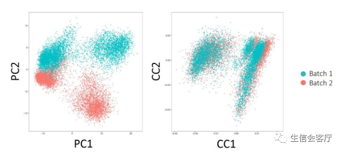
1、使用CCA分析将两个数据集降维到同一个低维空间,因为CCA降维之后的空间距离不是相似性而是相关性,所以相同类型与状态的细胞可以克服技术偏倚重叠在一起。CCA分析效果见下图:
2、CCA降维之后细胞在低维空间有了可以度量的“距离”,MNN(mutual nearest neighbor)算法以此找到两个数据集之间互相“距离”最近的细胞,Seurat将这些相互最近邻细胞称为“锚点细胞”。我们用两个数据集A和B来说明锚点,假设:
- A样本中的细胞A3与B样本中距离最近的细胞有3个(B1,B2,B3)
- B样本中的细胞B1与A样本中距离最近的细胞有4个(A1,A2,A3,A4)
- B样本中的细胞B2与A样本中距离最近的细胞有2个(A5,A6)
- B样本中的细胞B3与A样本中距离最近的细胞有3个(A1,A2,A7)
那么A3与B1是相互最近邻细胞,A3与B2、B3不是相互最近邻细胞,A3 B1就是A、B两个数据集中的锚点之一。实际数据中,两个数据集之间的锚点可能有几百上千个,如下图所示:
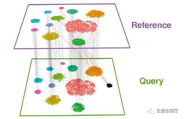
图中每条线段连接的都是相互最近邻细胞
3、理想情况下相同类型和状态的细胞才能构成配对锚点细胞,但是异常的情况也会出现,如上图中query数据集中黑色的细胞团。它在reference数据集没有相同类型的细胞,但是它也找到了锚点配对细胞(红色连线)。Seurat会通过两步过滤这些不正确的锚点:
- 在CCA低维空间找到的锚点,返回到基因表达数据构建的高维空间中验证,如果它们的转录特征相似性高则保留,否则过滤此锚点。
- 检查锚点细胞所在数据集最邻近的30个细胞,查看它们重叠的锚点配对细胞的数量,重叠越多分值越高,代表锚点可靠性更高。原理见下图:
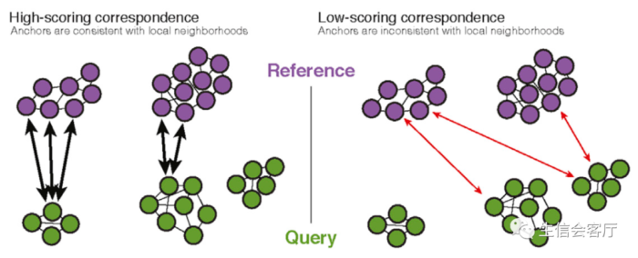
左边query数据集的一个锚点细胞能在reference数据集邻近区域找到多个配对锚点细胞,可以得到更高的锚点可靠性评分;右边一个锚点细胞只能在reference数据集邻近区域找到一个配对锚点细胞,锚点可靠性评分则较低。
4、经过层层过滤剩下的锚点细胞对,可以认为它们是相同类型和状态的细胞,它们之间的基因表达差异是技术偏倚引起的。Seurat计算它们的差异向量,然后用此向量校正这个锚点锚定的细胞子集的基因表达值。校正后的基因表达值即消除了技术偏倚,实现了两个单细胞数据集的整合。
library(Seurat)
library(tidyverse)
library(patchwork)
dir.create('cluster1')
dir.create('cluster2')
dir.create('cluster3')
set.seed(123) #设置随机数种子,使结果可重复
##==合并数据集==##
##使用目录向量合并
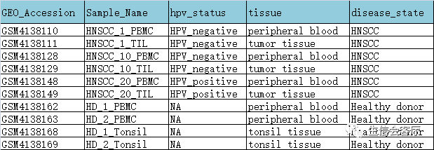
dir = c('data/GSE139324_HNC/GSM4138110',
'data/GSE139324_HNC/GSM4138111',
'data/GSE139324_HNC/GSM4138128',
'data/GSE139324_HNC/GSM4138129',
'data/GSE139324_HNC/GSM4138148',
'data/GSE139324_HNC/GSM4138149',
'data/GSE139324_HNC/GSM4138162',
'data/GSE139324_HNC/GSM4138163',
'data/GSE139324_HNC/GSM4138168',
'data/GSE139324_HNC/GSM4138169')
names(dir) = c('HNC01PBMC', 'HNC01TIL', 'HNC10PBMC', 'HNC10TIL', 'HNC20PBMC',
'HNC20TIL', 'PBMC1', 'PBMC2', 'Tonsil1', 'Tonsil2')
counts <- Read10X(data.dir = dir)
scRNA1 = CreateSeuratObject(counts, min.cells=1)
dim(scRNA1) #查看基因数和细胞总数
#[1] 23603 19750
table(scRNA1@meta.data$orig.ident) #查看每个样本的细胞数
#HNC01PBMC HNC01TIL HNC10PBMC HNC10TIL HNC20PBMC HNC20TIL PBMC1 PBMC2 Tonsil1 Tonsil2
# 1725 1298 1750 1384 1530 1148 2445 2436 3325 2709
#使用merge函数合并seurat对象
scRNAlist <- list()
#以下代码会把每个样本的数据创建一个seurat对象,并存放到列表scRNAlist里
for(i in 1:length(dir)){
counts <- Read10X(data.dir = dir[i])
scRNAlist[[i]] <- CreateSeuratObject(counts, min.cells=1)
}
#使用merge函数讲10个seurat对象合并成一个seurat对象
scRNA2 <- merge(scRNAlist[[1]], y=c(scRNAlist[[2]], scRNAlist[[3]],
scRNAlist[[4]], scRNAlist[[5]], scRNAlist[[6]], scRNAlist[[7]],
scRNAlist[[8]], scRNAlist[[9]], scRNAlist[[10]]))
#dim(scRNA2)
[1] 23603 19750
table(scRNA2@meta.data$orig.ident)
#HNC01PBMC HNC01TIL HNC10PBMC HNC10TIL HNC20PBMC HNC20TIL PBMC1 PBMC2 Tonsil1 Tonsil2
# 1725 1298 1750 1384 1530 1148 2445 2436 3325 2709scRNA1 <- NormalizeData(scRNA1)
scRNA1 <- FindVariableFeatures(scRNA1, selection.method = "vst")
scRNA1 <- ScaleData(scRNA1, features = VariableFeatures(scRNA1))
scRNA1 <- RunPCA(scRNA1, features = VariableFeatures(scRNA1))
plot1 <- DimPlot(scRNA1, reduction = "pca", group.by="orig.ident")
plot2 <- ElbowPlot(scRNA1, ndims=30, reduction="pca")
plotc <- plot1 plot2
ggsave("cluster1/pca.png", plot = plotc, width = 8, height = 4)
print(c("请选择哪些pc轴用于后续分析?示例如下:","pc.num=1:15"))
#选取主成分
pc.num=1:30
##细胞聚类
scRNA1 <- FindNeighbors(scRNA1, dims = pc.num)
scRNA1 <- FindClusters(scRNA1, resolution = 0.5)
table(scRNA1@meta.data$seurat_clusters)
metadata <- scRNA1@meta.data
cell_cluster <- data.frame(cell_ID=rownames(metadata), cluster_ID=metadata$seurat_clusters)
write.csv(cell_cluster,'cluster1/cell_cluster.csv',row.names = F)
##非线性降维
#tSNE
scRNA1 = RunTSNE(scRNA1, dims = pc.num)
embed_tsne <- Embeddings(scRNA1, 'tsne') #提取tsne图坐标
write.csv(embed_tsne,'cluster1/embed_tsne.csv')
#group_by_cluster
plot1 = DimPlot(scRNA1, reduction = "tsne", label=T)
ggsave("cluster1/tSNE.png", plot = plot1, width = 8, height = 7)
#group_by_sample
plot2 = DimPlot(scRNA1, reduction = "tsne", group.by='orig.ident')
ggsave("cluster1/tSNE_sample.png", plot = plot2, width = 8, height = 7)
#combinate
plotc <- plot1 plot2
ggsave("cluster1/tSNE_cluster_sample.png", plot = plotc, width = 10, height = 5)
#UMAP
scRNA1 <- RunUMAP(scRNA1, dims = pc.num)
embed_umap <- Embeddings(scRNA1, 'umap') #提取umap图坐标
write.csv(embed_umap,'cluster1/embed_umap.csv')
#group_by_cluster
plot3 = DimPlot(scRNA1, reduction = "umap", label=T)
ggsave("cluster1/UMAP.png", plot = plot3, width = 8, height = 7)
#group_by_sample
plot4 = DimPlot(scRNA1, reduction = "umap", group.by='orig.ident')
ggsave("cluster1/UMAP.png", plot = plot4, width = 8, height = 7)
#combinate
plotc <- plot3 plot4
ggsave("cluster1/UMAP_cluster_sample.png", plot = plotc, width = 10, height = 5)
#合并tSNE与UMAP
plotc <- plot2 plot4 plot_layout(guides = 'collect')
ggsave("cluster1/tSNE_UMAP.png", plot = plotc, width = 10, height = 5)
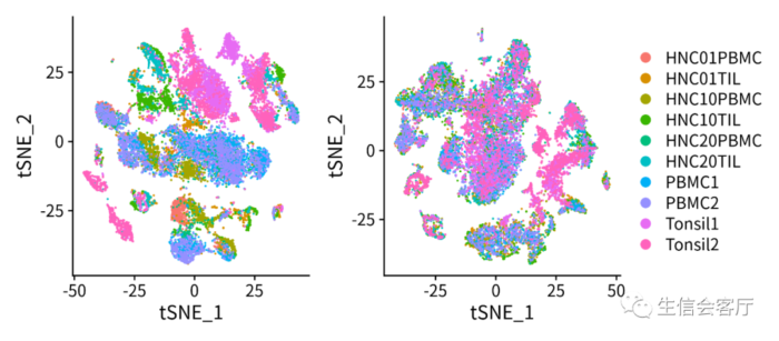
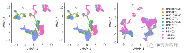
##scRNA2对象的降维聚类参考scRNA1的代码第一种方法合并数据的结果:
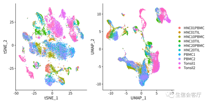
第二种方法合并数据的结果:

通过降维图可以看出两种方法的结果完全一致。这两种方法真的没有一点差异吗,有兴趣的朋友可以用GSE125449的数据集试试。
#scRNAlist是之前代码运行保存好的seurat对象列表,保存了10个样本的独立数据
#数据整合之前要对每个样本的seurat对象进行数据标准化和选择高变基因
for (i in 1:length(scRNAlist)) {
    scRNAlist[[i]] <- NormalizeData(scRNAlist[[i]])
    scRNAlist[[i]] <- FindVariableFeatures(scRNAlist[[i]], selection.method = "vst")
}
##以VariableFeatures为基础寻找锚点,运行时间较长
scRNA.anchors <- FindIntegrationAnchors(object.list = scRNAlist)
##利用锚点整合数据,运行时间较长
scRNA3 <- IntegrateData(anchorset = scRNA.anchors)
dim(scRNA3)
#[1]  2000 19750
#有没有发现基因数据只有2000个了?这是因为seurat整合数据时只用2000个高变基因。
#降维聚类的代码省略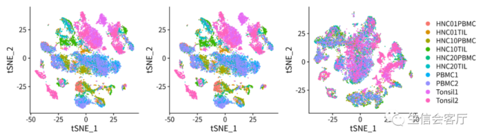
##==数据质控==#
scRNA <- scRNA3 #以后的分析使用整合的数据进行
##meta.data添加信息
proj_name <- data.frame(proj_name=rep("demo2",ncol(scRNA)))
rownames(proj_name) <- row.names(scRNA@meta.data)
scRNA <- AddMetaData(scRNA, proj_name)
##切换数据集
DefaultAssay(scRNA) <- "RNA"
##计算线粒体和红细胞基因比例
scRNA[["percent.mt"]] <- PercentageFeatureSet(scRNA, pattern = "^MT-")
#计算红细胞比例
HB.genes <- c("HBA1","HBA2","HBB","HBD","HBE1","HBG1","HBG2","HBM","HBQ1","HBZ")
HB_m <- match(HB.genes, rownames(scRNA@assays$RNA))
HB.genes <- rownames(scRNA@assays$RNA)[HB_m]
HB.genes <- HB.genes[!is.na(HB.genes)]
scRNA[["percent.HB"]]<-PercentageFeatureSet(scRNA, features=HB.genes)
#head(scRNA@meta.data)
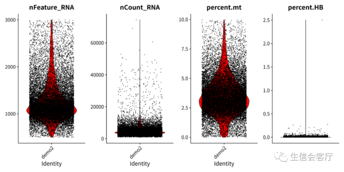
col.num <- length(levels(as.factor(scRNA@meta.data$orig.ident)))
##绘制小提琴图
#所有样本一个小提琴图用group.by="proj_name",每个样本一个小提琴图用group.by="orig.ident"
violin <-VlnPlot(scRNA, group.by = "proj_name",
features = c("nFeature_RNA", "nCount_RNA", "percent.mt","percent.HB"),
cols =rainbow(col.num),
pt.size = 0.01, #不需要显示点,可以设置pt.size = 0
ncol = 4)
theme(axis.title.x=element_blank(), axis.text.x=element_blank(), axis.ticks.x=element_blank())
ggsave("QC/vlnplot_before_qc.pdf", plot = violin, width = 12, height = 6)
ggsave("QC/vlnplot_before_qc.png", plot = violin, width = 12, height = 6)
plot1 <- FeatureScatter(scRNA, feature1 = "nCount_RNA", feature2 = "percent.mt")
plot2 <- FeatureScatter(scRNA, feature1 = "nCount_RNA", feature2 = "nFeature_RNA")
plot3 <- FeatureScatter(scRNA, feature1 = "nCount_RNA", feature2 = "percent.HB")
pearplot <- CombinePlots(plots = list(plot1, plot2, plot3), nrow=1, legend="none")
ggsave("QC/pearplot_before_qc.pdf", plot = pearplot, width = 12, height = 5)
ggsave("QC/pearplot_before_qc.png", plot = pearplot, width = 12, height = 5)
##设置质控标准
print(c("请输入允许基因数和核糖体比例,示例如下:", "minGene=500", "maxGene=4000", "pctMT=20"))
minGene=500
maxGene=3000
pctMT=10
##数据质控
scRNA <- subset(scRNA, subset = nFeature_RNA > minGene & nFeature_RNA < maxGene & percent.mt < pctMT)
col.num <- length(levels(as.factor(scRNA@meta.data$orig.ident)))
violin <-VlnPlot(scRNA, group.by = "proj_name",
features = c("nFeature_RNA", "nCount_RNA", "percent.mt","percent.HB"),
cols =rainbow(col.num),
pt.size = 0.1,
ncol = 4)
theme(axis.title.x=element_blank(), axis.text.x=element_blank(), axis.ticks.x=element_blank())
ggsave("QC/vlnplot_after_qc.pdf", plot = violin, width = 12, height = 6)
ggsave("QC/vlnplot_after_qc.png", plot = violin, width = 12, height = 6)质控后的数据
为了后续分析的方便,我们先用SingleR预测每个cluster的细胞类型。
##==鉴定细胞类型==##
library(SingleR)
dir.create("CellType")
refdata <- MonacoImmuneData()
testdata <- GetAssayData(scRNA, slot="data")
clusters <- scRNA@meta.data$seurat_clusters
#使用Monaco参考数据库鉴定
cellpred <- SingleR(test = testdata, ref = refdata, labels = refdata$label.main,
                     method = "cluster", clusters = clusters,
                     assay.type.test = "logcounts", assay.type.ref = "logcounts")
celltype = data.frame(ClusterID=rownames(cellpred), celltype=cellpred$labels, stringsAsFactors = F)
write.csv(celltype,"CellType/celltype_Monaco.csv",row.names = F)
scRNA@meta.data$celltype_Monaco = "NA"
for(i in 1:nrow(celltype)){
scRNA@meta.data[which(scRNA@meta.data$seurat_clusters == celltype$ClusterID[i]),'celltype_Monaco'] <- celltype$celltype[i]}
p1 = DimPlot(scRNA, group.by="celltype_Monaco", repel=T, label=T, label.size=5, reduction='tsne')
p2 = DimPlot(scRNA, group.by="celltype_Monaco", repel=T, label=T, label.size=5, reduction='umap')
p3 = p1 p2  plot_layout(guides = 'collect')
ggsave("CellType/tSNE_celltype_Monaco.png", p1, width=7 ,height=6)
ggsave("CellType/UMAP_celltype_Monaco.png", p2, width=7 ,height=6)
ggsave("CellType/celltype_Monaco.png", p3, width=10 ,height=5)
#使用DICE参考数据库鉴定
refdata <- DatabaseImmuneCellExpressionData()
# load('~/database/SingleR_ref/ref_DICE_1561s.RData')
# refdata <- ref_DICE
testdata <- GetAssayData(scRNA, slot="data")
clusters <- scRNA@meta.data$seurat_clusters
cellpred <- SingleR(test = testdata, ref = refdata, labels = refdata$label.main,
                     method = "cluster", clusters = clusters,
                     assay.type.test = "logcounts", assay.type.ref = "logcounts")
celltype = data.frame(ClusterID=rownames(cellpred), celltype=cellpred$labels, stringsAsFactors = F)
write.csv(celltype,"CellType/celltype_DICE.csv",row.names = F)
scRNA@meta.data$celltype_DICE = "NA"
for(i in 1:nrow(celltype)){
scRNA@meta.data[which(scRNA@meta.data$seurat_clusters == celltype$ClusterID[i]),'celltype_DICE'] <- celltype$celltype[i]}
p4 = DimPlot(scRNA, group.by="celltype_DICE", repel=T, label=T, label.size=5, reduction='tsne')
p5 = DimPlot(scRNA, group.by="celltype_DICE", repel=T, label=T, label.size=5, reduction='umap')
p6 = p3 p4  plot_layout(guides = 'collect')
ggsave("CellType/tSNE_celltype_DICE.png", p4, width=7 ,height=6)
ggsave("CellType/UMAP_celltype_DICE.png", p5, width=7 ,height=6)
ggsave("CellType/celltype_DICE.png", p6, width=10 ,height=5)
#对比两种数据库鉴定的结果
p8 = p1 p4
ggsave("CellType/Monaco_DICE.png", p8, width=12 ,height=5)

##保存数据
saveRDS(scRNA,'scRNA.rds')
用两个参考数据库分别运行SingleR,结果有一定差异,由此可见SingleR Marker基因人工鉴定才是可靠的细胞鉴定的方法。
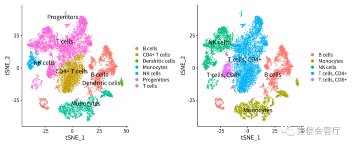
我们后续分析采用左图鉴定的结果