

1. 背景知识
本章我们将用一个具体案例来介绍用R语言构建Logistic回归预测模型并绘制Nomogram的完整过程。有关预测模型的构建流程我们将在下一章《预测模型系列04–基于R的生存资料预测模型构建与Nomogram绘制》中介绍;有关预测模型优劣的评价方法我们将在后续章节中介绍。我们可以把临床预测模型构建与验证的步骤总结为以下7个步骤:
(1)明确临床问题,确定科学假说
(2)根据既往文献,确定预测模型研究思路
(3)确定预测模型的预测变量
(4)确定预测模型的结局变量
(5)构建预测模型,计算模型预测值
(6)模型区分能力评估
(7)模型的准确性评估
其中步骤2有关预测模型的研究思路,大家可以参见本文图1.
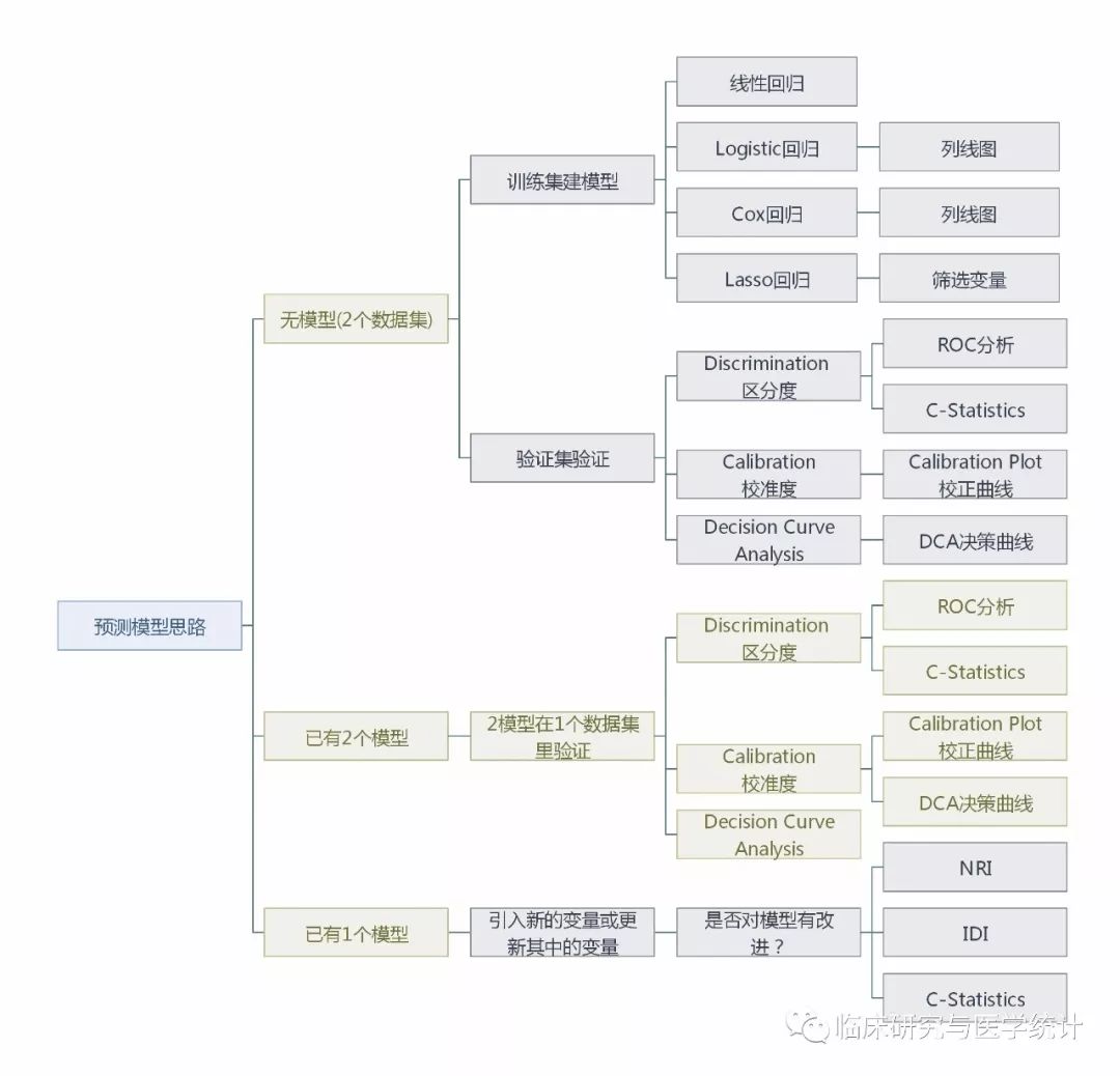
图1.三种预测模型的研究思路
2. 案例分析
Hosmer和 Lemeshow于1989年研究了低出生体重婴儿的影响因素。结果变量为:是否娩出低出生体重儿(变量名为“low”,二分类变量,1=低出生体重,即婴儿出生体重<2500g;0=非低出生体重),考虑的影响因素(自变量)有:产妇妊娠前体重(lwt,磅);产妇年龄(age,岁);产妇在妊娠期间是否吸烟(smoke,0=未吸、1=吸烟);本次妊娠前早产次数(ptl,次);是否患有高血压(ht,0=未患、1=患病);子宫对按摩、催产素等刺激引起收缩的应激性(ui,0=无、1=有);妊娠前三个月社区医生随访次数(ftv,次);种族(race,1=白人、2=黑人、3=其他民族)。本案例因变量是二分类变量(是否低出生体重儿),研究目的是探讨低出生体重儿的独立影响因素,符合二元Logistic回归的应用条件。因为本例中,我们只有这一个数据集,可以用这个数据集作为训练集建模,然后在本数据集利用Bootstrap重抽样的方法进行模型验证。下面我们就基于R语言演示预测低出生体重儿的预测模型构建与Nomogram的绘制,我们把数据sav的数据格式整理好,命名为“lweight.sav”,保存在R语言当前工作路径下。具体分析步骤如下:
(1)首先筛选影响低出生体重儿的独立影响因素,构建Logistic回归模型;
(2)绘制Nomogram;
(3)计算模型的区分度 C-Statistics;
(4)重抽样的方法进行模型验证,并绘制Calibration曲线。
3.代码及结果解读
载入foreign包用于导入sav格式的数据;载入rms包用于构建logistics回归模型,绘制列线图:
library(foreign)
library(rms)## Loading required package: Hmisc## Loading required package: lattice## Loading required package: survival## Loading required package: Formula## Loading required package: ggplot2## Attaching package: 'Hmisc'## The following objects are masked from 'package:base':
##
##     format.pval, units## Loading required package: SparseM## Attaching package: 'SparseM'## The following object is masked from 'package:base':
##
##     backsolve
导入sav格式的数据,把数据设置为数据框结构,并展示数据的前6行。
mydata<-read.spss("lweight.sav")
mydata<-as.data.frame(mydata)
head(mydata)##   id      low age lwt     race  smoke ptl       ht ui ftv  bwt
## 1 85 正常体重  19 182   黑种人 不吸烟   0 无妊高症 有   0 2523
## 2 86 正常体重  33 155 其他种族 不吸烟   0 无妊高症 无   3 2551
## 3 87 正常体重  20 105   白种人   吸烟   0 无妊高症 无   1 2557
## 4 88 正常体重  21 108   白种人   吸烟   0 无妊高症 有   2 2594
## 5 89 正常体重  18 107   白种人   吸烟   0 无妊高症 有   0 2600
## 6 91 正常体重  21 124 其他种族 不吸烟   0 无妊高症 无   0 2622
数据预处理,设置结局变量为二分类,并对“race”变量设置哑变量
mydata$low <- ifelse(mydata$low =="低出生体重",1,0)
mydata$race1 <- ifelse(mydata$race =="白种人",1,0)
mydata$race2 <- ifelse(mydata$race =="黑种人",1,0)
mydata$race3 <- ifelse(mydata$race =="其他种族",1,0)
把数据框加载到当前工作环境,datadist()打包数据
attach(mydata)
dd<-datadist(mydata)
options(datadist='dd')
拟合模型,并展示模型拟合的结果与模型参数。注意:可直接读取模型中Rank Discrim.参数 C,即为fit1模型的C-statistics。
fit1<-lrm(low~age+ftv+ht+lwt+ptl+smoke+ui+race1+race2,data=mydata,x=T,y=T)
fit1## Logistic Regression Model
##
##  lrm(formula = low ~ age + ftv + ht + lwt + ptl + smoke + ui +
##      race1 + race2, data = mydata, x = T, y = T)
##
##                       Model Likelihood     Discrimination    Rank Discrim.
##                          Ratio Test           Indexes           Indexes
##  Obs           189    LR chi2     31.12    R2       0.213    C       0.738
##   0            130    d.f.            9    g        1.122    Dxy     0.476
##   1             59    Pr(> chi2) 0.0003    gr       3.070    gamma   0.477
##  max |deriv| 7e-05                         gp       0.207    tau-a   0.206
##                                            Brier    0.181
##
##             Coef    S.E.   Wald Z Pr(>|Z|)
##  Intercept   1.1427 1.0873  1.05  0.2933
##  age        -0.0255 0.0366 -0.69  0.4871
##  ftv         0.0321 0.1708  0.19  0.8509
##  ht=妊高症   1.7631 0.6894  2.56  0.0105
##  lwt        -0.0137 0.0068 -2.02  0.0431
##  ptl         0.5517 0.3446  1.60  0.1094
##  smoke=吸烟  0.9275 0.3986  2.33  0.0200
##  ui=有       0.6488 0.4676  1.39  0.1653
##  race1      -0.9082 0.4367 -2.08  0.0375
##  race2       0.3293 0.5339  0.62  0.5374
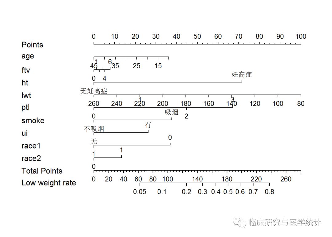
构建列线图对象nom1, 打印列线图,结果如下图所示。
nom1 <- nomogram(fit1, fun=plogis,fun.at=c(.001, .01, .05, seq(.1,.9, by=.1), .95, .99, .999),lp=F, funlabel="Low weight rate")
plot(nom1)
构建校准曲线对象cal1,打印校准曲线,结果如下。
cal1 <- calibrate(fit1, method='boot', B=1000)
plot(cal1,xlim=c(0,1.0),ylim=c(0,1.0))
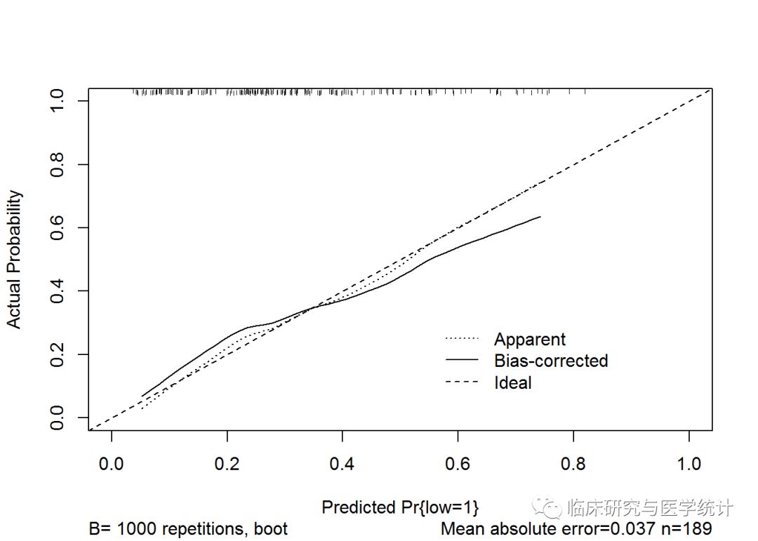
## n=189   Mean absolute error=0.037   Mean squared error=0.00184
## 0.9 Quantile of absolute error=0.055
从以上Logistics回归模型fit1的计算结果以及图2.不难看出我们纳入模型中的有些预测变量对于模型的贡献可以忽略不计,比如变量“ftv”,还有一些预测变量比如“race”通过设置哑变量的形式进入预测模型可能并不合适,临床操作繁琐,我们可以考虑将无序分类变量适当转换为二分类变量纳入回归模型。调整后代码如下:
把无序分类变量设置为二分类变量
mydata$race <- as.factor(ifelse(mydata$race=="白种人", "白种人","黑人及其他种族"))
模型中排除额变量ftv重新建模fit2
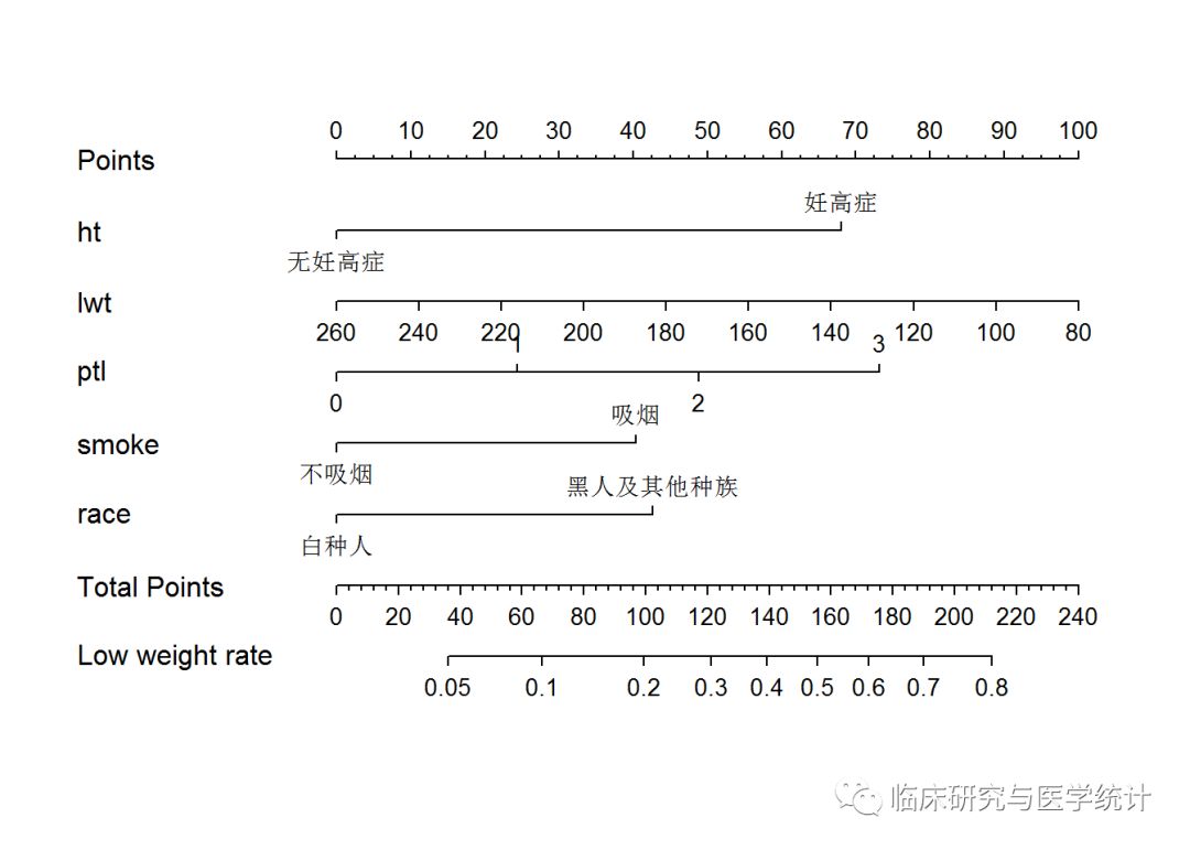
dd<-datadist(mydata)
options(datadist='dd')
fit2<-lrm(low~ht+lwt+ptl+smoke+race,data=mydata,x=T,y=T)
fit2
## Logistic Regression Model
##
##  lrm(formula = low ~ ht + lwt + ptl + smoke + race, data = mydata,
##      x = T, y = T)
##
##                        Model Likelihood     Discrimination    Rank Discrim.
##                           Ratio Test           Indexes           Indexes
##  Obs           189    LR chi2      28.19    R2       0.195    C       0.732
##   0            130    d.f.             5    g        1.037    Dxy     0.465
##   1             59    Pr(> chi2) <0.0001    gr       2.820    gamma   0.467
##  max |deriv| 1e-05                          gp       0.194    tau-a   0.201
##                                             Brier    0.184
##
##                      Coef    S.E.   Wald Z Pr(>|Z|)
##  Intercept           -0.2744 0.8832 -0.31  0.7561
##  ht=妊高症            1.6754 0.6863  2.44  0.0146
##  lwt                 -0.0137 0.0064 -2.14  0.0322
##  ptl                  0.6006 0.3342  1.80  0.0723
##  smoke=吸烟           0.9919 0.3869  2.56  0.0104
##  race=黑人及其他种族  1.0487 0.3842  2.73  0.0063
nom2 <- nomogram(fit2, fun=plogis,fun.at=c(.001, .01, .05, seq(.1,.9, by=.1), .95, .99, .999),lp=F, funlabel="Low weight rate")
plot(nom2)
cal2 <- calibrate(fit2, method='boot', B=1000)
plot(cal2,xlim=c(0,1.0),ylim=c(0,1.0))
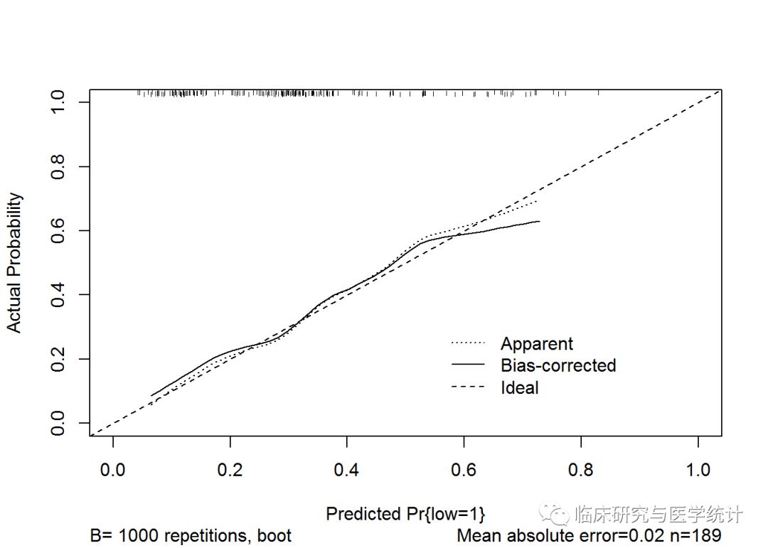
## n=189   Mean absolute error=0.02   Mean squared error=0.00066
## 0.9 Quantile of absolute error=0.033
4. 总结与讨论
综上,本文介绍了Logistic回归预测模型构建以及Nomogram的绘制。需要说明的是一个预测模型是否具有较好的实际运用价值,除了考量其预测的准确性还要考量其可操作性。除了内部验证检验其准确性,外部验证有时也是必须的,本例中因未获得较好的外部验证数据及并未演示外部验证的操作过程,仅用Bootstrap的方法在原有数据集进行了验证。
5. 参考文献
[1].周支瑞,胡志德.聪明统计学. 长沙:中南大学出版社, 2016.
[2].周支瑞,胡志德.疯狂统计学. 长沙:中南大学出版社, 2018.
1F
请问在二项logistic回归中glm函数和lrm函数的用法是等价的吗?可以同时使用吗