基因表达分析（上）

来源：hoptop1 4,242

本系列教程包括：

基因表达分析（上）

基因表达分析（中）

基因表达分析（下）

还在利用hisat, tophat这些耳熟能详的软件将read比对到基因组（转录组）上，然后统计每个基因的count数么？试试这些不需要比对，速度更快的工具吧。

Salmon(Patro et al. 2016),
Sailfish (Patro, Mount, and Kingsford 2014)
kallisto (Bray et al. 2016)
RSEM(B. Li and Dewey 2011)

这里就介绍一下Salmon工具，文章发表在nature method，如下是摘要

We introduce Salmon, a lightweight method for quantifying transcript abundance from RNA–seq reads. Salmon combines a new dual-phase parallel inference algorithm and feature-rich bias models with an ultra-fast read mapping procedure. It is the first transcriptome-wide quantifier to correct for fragment GC-content bias, which, as we demonstrate here, substantially improves the accuracy of abundance estimates and the sensitivity of subsequent differential expression analysis.

谁能给我解释下：

dual-phase parallel interence algorithm
feature-rich bias modesl

算法这个东西，目前还不是我能力范围所能掌控的。反正他说他能让丰度预测更加准确，让后续的差异表达分析更加敏感。作者认为目前的工具都缺少样本特异性误差模型，然后我用了新的模型弥补了这个缺陷。(好吧，你最棒了)

existing methods for transcriptome-wide abundance estimation—both alignment-based and alignment-free—lack sample-specific bias models rich enough to capture important effects like fragment GC-content bias. When correction is not applied, these biases can lead to undesired effects, for example, a loss of false discovery rate (FDR) control in differential expression studies5.existing methods for transcriptome-wide abundance estimation—both alignment-based and alignment-free—lack sample-specific bias models rich enough to capture important effects like fragment GC-content bias. When correction is not applied, these biases can lead to undesired effects, for example, a loss of false discovery rate (FDR) control in differential expression studies⁵.

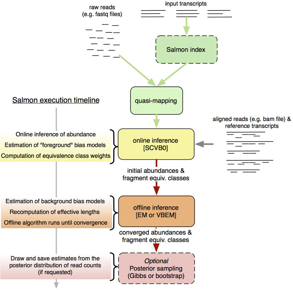
最后放一张Salmon的流程图，大家意会吧。

Overview of Salmon/'s method and components and execution timeline.

安装

Salmon非常贴心的提供了二进制版本，所以可以在https://github.com/COMBINE-lab/salmon/releases 下载最新的版本，当然你可以选择下载source code，然后自己编译。

我习惯把软件放到家目录下的biosoft文件夹下，然后把程序的路径存放到PATH中，最后的效果如下：

$ salmon -h
Salmon v0.8.2

Usage:  salmon -h|--help or
        salmon -v|--version or
        salmon -c|--cite or
        salmon [--no-version-check] <COMMAND> [-h | options]

Commands:
     cite  Show salmon citation information
     index Create a salmon index
     quant Quantify a sample
     swim  Perform super-secret operation

简单说明

Salmon提供了官方文档http://salmon.readthedocs.io/en/latest/, 所以哪里不懂就去这里先看，如果解决不了问题，就去Google（不知道如何上Google，请百度如何上Google）。

Salmon的输入数据可以分为两种：

参考转录组（记住是转录组，而不是全基因组）和你的测序结果（FASTA/FASTQ格式）
已比对文件（SAM/BAM)和参考转录组（记住是转录组，而不是全基因组，好了，你别说了，我记住了）

根据输入数据不同，分为两种模式

quasi-mapping-based mode
alignment-based mode

以Salmon自带的测试数据为例(解压sample_data.tar.tgz可得)：

$ ls
reads_1.fastq  reads_2.fastq  transcripts.fasta

第一步：要建立参考转录组的索引（记住是转录组，而不是全基因组，好了！你别说了，我记住了）

salmon index -t transcripts.fasta -i transcripts_index --type quasi -k 31

# 参数说明
-t： 输入的参考转录组名（记住是转录组，而不是全基因组，好了！你别说了，我记住了）
-i： 输出index的名字
-type： 索引类型，分为fmd, quasi, 建议quasi
-k: k-mers的长度。read长度大于75bp， 作者建议31

第二步：对RNA测序结果进行定量

salmon quant -i transcripts_index  -l A -1 reads_1.fastq -2 reads_2.fastq -o transcripts_quant

# 参数解释
-i： 输入之前的index路径
-l/--libType: 文库类型，请看后续的文档
-1： read1，支持压缩文件
-2： read2，支持压缩文件
-o： 输出目录

文库具体说明，见官方文档：http://salmon.readthedocs.io/en/latest/salmon.html#what-s-this-libtype。尽管你可以用-A程序自动决定，但是了解不同的文库类型可以帮助你理解-A是如何发挥功能。

输出的结果如下：

$ ls
aux_info  cmd_info.json  lib_format_counts.json  libParams  logs  quant.sf
$ head quant.sf
Name    Length  EffectiveLength TPM     NumReads
NM_001168316    2283    2105.89 12603.4 160.897
NM_174914       2385    2207.89 112095  1500.32
NR_031764       1853    1675.89 10117.2 102.785
NM_004503       1681    1503.89 36217.5 330.184
NM_006897       1541    1363.89 80309.5 664
NM_014212       2037    1859.89 4878.13 55
NM_014620       2300    2122.89 45827   589.754
NM_017409       1959    1781.89 4351.06 47
NM_017410       2396    2218.89 3122.42 42

第三步：将结果导入R
接着可以用DESeq2的txmport将处理结果导入R，

txi.salmon <- tximport('quant.sf', type = "salmon", tx2gene = tx2gene)

现实中的数据

演示的数据来自于发表在Nature commmunication 上的一篇文章 “Temporal dynamics of gene expression and histone marks at the Arabidopsis shoot meristem during flowerin”。原文用RNA-Seq的方式研究在开花阶段,芽分生组织在不同时期的基因表达变化。

原文的流程是： TopHat -> SummarizeOverlaps -> Deseq2 -> AmiGO
其中比对的参考基因组为TAIR10 ver.24 ，并且屏蔽了ribosomal RNA
regions (2:3471–9557; 3:14,197,350–14,203,988)。Deseq2只计算至少在一个时间段的FPKM的count > 1 的基因。

数据存放在http://www.ebi.ac.uk/arrayexpress/, ID为E-MTAB-5130。

实验设计： 4个时间段（0,1,2,3），分别有4个生物学重复，一共有16个样品。

数据下载

首先下载数据说明文件：

$ wget http://www.ebi.ac.uk/arrayexpress/files/E-MTAB-5130/E-MTAB-5130.sdrf.txt

然后根据数据说明文件提供的FTP链接下载

$ head -n1 E-MTAB-5130.sdrf.txt | tr '\t' '\n' | nl | grep URI
    33  Comment[FASTQ_URI]
    
$ tail -n +2 E-MTAB-5130.sdrf.txt | cut -f 33 | xargs -i wget {}

根据下载速度，你们可以选择去吃吃饭，还是睡睡觉。

下载完RNA-Seq数据后，我们还需要下载一个拟南芥cDNA序列(记住是转录组，而不是全基因组，好了，你别说了，我记住了)

$ curl ftp://ftp.ensemblgenomes.org/pub/plants/release-28/fasta/arabidopsis_thaliana/cdna/Arabidopsis_thaliana.TAIR10.28.cdna.all.fa.gz -o athal.fa.gz

然后用Salmon建立索引：

salmon index -t athal.fa.gz -i athal_index

数据定量

由于样本一共有16个，不可能一条条输入命令，所以我们写一个脚本：

#! /bin/bash
for fn in ERR1698{194..209};
do
    samp=`basename ${fn}`
    echo "Processin sample ${sampe}"
    salmon quant -i athal_index -l A \
        -1 ${samp}_1.fastq.gz \
        -2 ${samp}_2.fastq.gz \
        -p 8 -o quants/${samp}_quant
done

根据你电脑的配置，你可以选择吃下午茶，还是选择睡个午觉。

数据导入R

当然你完全不必真的去睡午觉，我们可以程序运行的时候准备一下tximport所需要的输入文件。

tximport可以纠正不同样本基因长度的潜在改变（比如说differential isoform usage）；能够用于导入 (Salmon, Sailfish, kallisto)程序的输出文件；能够避免丢弃那些比对到多个基因的同源序列，从而提高灵敏度

In particular, the tximport pipeline offers the following benefits: (i) this approach corrects for potential changes in gene length across samples (e.g. from differential isoform usage) (Trapnell et al. 2013), (ii) some of the upstream quantification methods (Salmon, Sailfish, kallisto) are substantially faster and require less memory and disk usage compared to alignment-based methods that require creation and storage of BAM files, and (iii) it is possible to avoid discarding those fragments that can align to multiple genes with homologous sequence, thus increasing sensitivity (Robert and Watson 2015)

虽然tximport的参数看起来很多，但其实需要我们准备的就是两个files和tx2gene

tximport(files, type = c("none", "salmon", "sailfish", "kallisto", "rsem"),
  txIn = TRUE, txOut = FALSE, countsFromAbundance = c("no", "scaledTPM",
  "lengthScaledTPM"), tx2gene = NULL, varReduce = FALSE,
  dropInfReps = FALSE, ignoreTxVersion = FALSE, geneIdCol, txIdCol,
  abundanceCol, countsCol, lengthCol, importer = NULL)

files存放的是salmon的输出文件，所以我们需要根据文件存放位置，进行声明

dir <- "C:/Users/Xu/Desktop/"
list.files(dir)
sample <- paste0("ERR1698",seq(194,209),"_quant")
files <- file.path(dir,"quants",sample,"quant.sf")
names(files) <- paste0("sample",c(1:16))
all(file.exists(files))

然后我们还要准备一个基因名和转录本名字相关的数据框

library(AnnotationHub)
ah <- AnnotationHub()
ath <- query(ah,'thaliana')
ath_tx <- ath[['AH52247']]
columns(ath_tx)
k <- keys(ath_tx,keytype = "GENEID")
df <- select(ath_tx, keys=k, keytype = "GENEID",columns = "TXNAME")
tx2gene <- df[,2:1] # TXID在前， GENEID在后

如果你电脑跑的够快，基本上这个时候就可以导入数据了。

# install.packages("readr")
# install.packages("rsjon")
library("tximport")
library("readr")
txi <- tximport(files, type = "salmon", tx2gene = tx2gene)

# reading in files with read_tsv
# 1 2 3 4 5 6 7 8 9 10 11 12 13 14 15 16 
# summarizing abundance
# summarizing counts
# summarizing length

names(txi)
[1] "abundance"           "counts"              "length"             
[4] "countsFromAbundance

head(txi$lenght)
head(txi$counts)

由于后续要用DESeq2包做差异表达分析，所以需要用DESeqDataSetFromTximport这个函数，当然你还需要说明你的实验设计

library("DESeq2")
sampleTable <- data.frame(condition = factor(
  rep(c("Day0","Day1","Day2","Day3"),each=4)))
rownames(sampleTable) <- colnames(txi$counts)
dds <- DESeqDataSetFromTximport(txi, sampleTable, ~condition)

总结

使用Salmon对样本的转录水平进行定量
使用tximport导入数据
使用DESeqDataSetFromTximport将数据导入DESeq2

基因表达分析（上）

安装

简单说明

现实中的数据

数据下载

数据定量

数据导入R

总结

来自外部的引用

发表评论