

前面我们使用qplot函数对ggplot2做图的方法进行了初步的了解,并比较了qplot和plot函数的用法。从最终得到的结果(图形)来看,除了外观不同外好像qplot函数和plot函数并没有什么本质的差别。这其实是一个骗局!
1 图形对象
我们知道,R语言基本做图方法都是通过函数完成的(如果不了解请参考本博客《散点图》一文),这些函数直接在输出设备上执行一些列操作得到图形。很多函数没有返回值,即使有返回值也不会反映绘图操作的整个过程。但ggplot2不一样,它用图形对象存储做图的细节,通过输出图形对象获得图形。一行一行地运行下面代码可以发现这一点:
library(ggplot2)
theme_set(theme_bw())
x <- 1:100
y <- rnorm(100)
p1 <- plot(x, y)
p2 <- qplot(x, y)

很显然执行最后一行代码不会得到想要的图形。下面再看看 p1 和 p2 分别是什么:
class(p1)
## [1] "NULL"
class(p2)
## [1] "gg"     "ggplot"
typeof(p2)
## [1] "list"
str(p2)
## List of 9
##  $ data       :'data.frame': 0 obs. of  0 variables
##  $ layers     :List of 1
##   ..$ :Classes 'proto', 'environment'
##  $ scales     :Reference class 'Scales' [package "ggplot2"] with 1 fields
##   ..$ scales: list()
##   ..and 21 methods, of which 9 are possibly relevant:
##   ..  add, clone, find, get_scales, has_scale, initialize, input, n,
##   ..  non_position_scales
##  $ mapping    :List of 2
##   ..$ x: symbol x
##   ..$ y: symbol y
##  $ theme      : list()
##  $ coordinates:List of 1
##   ..$ limits:List of 2
##   .. ..$ x: NULL
##   .. ..$ y: NULL
##   ..- attr(*, "class")= chr [1:2] "cartesian" "coord"
##  $ facet      :List of 1
##   ..$ shrink: logi TRUE
##   ..- attr(*, "class")= chr [1:2] "null" "facet"
##  $ plot_env   :
##  $ labels     :List of 2
##   ..$ x: chr "x"
##   ..$ y: chr "y"
##  - attr(*, "class")= chr [1:2] "gg" "ggplot"
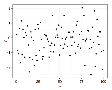
plot函数的返回值p1的class属性为NULL(空),而qplot函数的返回值p2的calss属性有两个“gg” 和 “ggplot”,其本质是长度为9的列表对象。打印这个对象就会得到图形:
print(p2)
qplot函数的作用是产生一个ggplot对象,但获得ggplot对象的更一般方法是使用对象类型的同名函数ggplot。它的用法是:
# 非运行代码
ggplot(df, aes(x, y, <other aesthetics>))
ggplot(df)
ggplot()
ggplot函数用于初始化一个ggplot对象,即使不指定任何做图相关的内容,它的结构也是完整的:
length(p2)
## [1] 9
length(ggplot())
## [1] 9
2 ggplot图形对象组成
ggplot图形对象是由9个元素组成的列表,这点已经清楚。元素的名称为:
names(p2)
## [1] "data"        "layers"      "scales"      "mapping"     "theme"
## [6] "coordinates" "facet"       "plot_env"    "labels"
但是单从图形对象的结构上没办法理解ggplot2做图的过程和细节,所以还得了解一点相关的理论。ggplot2是Wilkinson做图理论 Grammer of Graphics 的R语言实现。太高深了,不知道从哪开始,还是从ggplot图形列表对象的元素组成做一点简单了解吧。
2.1 数据 data
似乎就是数据。但是如果试图查看上面p2对象的数据:
p2$data
## data frame with 0 columns and 0 rows
是空的。但如果使用qplot函数时指定了data,情况就不一样了:
p3 <- qplot(carat, price, data=diamonds, color=cut, shape=cut)
head(p3$data, 3)
##   carat     cut color clarity depth table price    x    y    z
## 1  0.23   Ideal     E     SI2  61.5    55   326 3.95 3.98 2.43
## 2  0.21 Premium     E     SI1  59.8    61   326 3.89 3.84 2.31
## 3  0.23    Good     E     VS1  56.9    65   327 4.05 4.07 2.31
nrow(p3$data)
## [1] 53940
列表对象的data元素存储了整个diamnods数据框的数据。用ggplot函数可以单独指定data项:
p4 <- ggplot(diamonds)
head(p4$data, 3)
##   carat     cut color clarity depth table price    x    y    z
## 1  0.23   Ideal     E     SI2  61.5    55   326 3.95 3.98 2.43
## 2  0.21 Premium     E     SI1  59.8    61   326 3.89 3.84 2.31
## 3  0.23    Good     E     VS1  56.9    65   327 4.05 4.07 2.31
2.2 映射 mapping
ggplot对象的data项存储了整个数据框的内容,而“映射”则确定如何使用这些数据。在ggplot2中,图形的可视属性如形状、颜色、透明度等称为美学属性(或艺术属性),确定数据与美学属性之间对应关系的过程称为映射,通常使用aes函数完成(qplot函数中使用参数设置映射):
str(p3$mapping)
## List of 4
##  $ colour: symbol cut
##  $ shape : symbol cut
##  $ x     : symbol carat
##  $ y     : symbol price
str(p4$mapping)
##  list()
p4 <- p4 + aes(x=carat, y=price, color=color, shape=cut)
str(p4$mapping)
## List of 4
##  $ x     : symbol carat
##  $ y     : symbol price
##  $ colour: symbol color
##  $ shape : symbol cut
p4 <- p4 + aes(x=carat, y=price, color=cut, shape=cut)
str(p4$mapping)
## List of 4
##  $ x     : symbol carat
##  $ y     : symbol price
##  $ colour: symbol cut
##  $ shape : symbol cut
需要说明的是,上面第三行代码使用了加号,这是ggplot2为ggplot对象定义的运算方法,表示设置ggplot对象中对应的内容。
2.3 图层 layers
2.3.1 图层组成
在ggplot的列表结构里面看不到我们指定的图形类型参数。这些设置被分派到layers里面了:
p3$layers
## [[1]]
## geom_point:
## stat_identity:
## position_identity: (width = NULL, height = NULL)
一个图层包含了至少3个东西(数据和映射当然必需,另算):geom、stat和position
- 几何类型 geom:是数据在图上的展示形式,即点、线、面等。在ggplot2里面有很多预定义的几何类型。
- 统计类型 stat:是对数据所应用的统计类型/方法。上面的p2和p3对象我们并没有指定统计类型,但是自动获得了identity,因为ggplot2为每一种几何类型指定了一种默认的统计类型,反之亦然。所以如果仅指定geom或stat中的一个,另外一个会自动获取。
- 位置 position:几何对象在图像上的位置调整,这也有默认设定。
不指定几何类型或统计类型的ggplot对象的图层是空列表,即没有图层,也不能输出图像:
p4$layers
## list()
print(p4)
## Error: No layers in plot
也就是说,指定了几何类型或统计类型,图层就会产生:
(p4 + geom_point())$layers
## [[1]]
## geom_point: na.rm = FALSE
## stat_identity:
## position_identity: (width = NULL, height = NULL)
(p4 + stat_identity())$layers
## [[1]]
## geom_point:
## stat_identity: width = NULL, height = NULL
## position_identity: (width = NULL, height = NULL)
为什么图层说“至少”包含3个内容呢?如果你把整个图层的内容转成列表结构显示以下就会发现更多:
as.list((p4 + geom_point())$layers[[1]])
## $mapping
## NULL
##
## $geom_params
## $geom_params$na.rm
## [1] FALSE
##
##
## $stat_params
## named list()
##
## $stat
## stat_identity:
##
## $inherit.aes
## [1] TRUE
##
## $geom
## geom_point:
##
## $position
## position_identity: (width = NULL, height = NULL)
##
## $subset
## NULL
##
## $data
## list()
## attr(,"class")
## [1] "waiver"
##
## $show_guide
## [1] NA
2.3.2 图层加法
从图层的结构可以看到它在ggplot对象中是一个多重列表,如果对ggplot对象做图层加法运算,是增加图层而不是替换图层:
(p4 + geom_point() + geom_line())$layers
## [[1]]
## geom_point: na.rm = FALSE
## stat_identity:
## position_identity: (width = NULL, height = NULL)
##
## [[2]]
## geom_line:
## stat_identity:
## position_identity: (width = NULL, height = NULL)
2.3.3 图层顺序
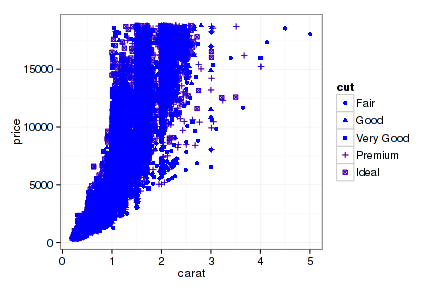
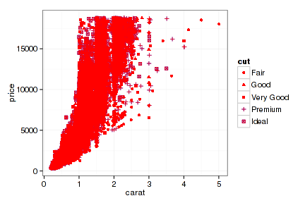
ggplot2按“层”做图,所以图层的顺序对于图形的表现会有影响,如果几何对象有叠加,那么后面图层的对象会覆盖前面图层的对象。下面只是调换了两个图层的顺序,但由于数据点是相同的,所以图形的颜色完全不一样:
p4 + geom_point(color="red") + geom_point(color="blue")
p4 + geom_point(color="blue") + geom_point(color="red")
2.4 标尺 scales
这是ggplot2中比较复杂的一个概念,从ggplot对象中能获取的信息不多:
p4$scales
## Reference class object of class "Scales"
## Field "scales":
## list()
在ggplot2中,一个标尺就是一个函数,它使用一系列参数将我们的数据(如钻石价格、克拉)转成计算机能够识别的数据(如像素、颜色值),然后展示在图像上。使用标尺对数据进行处理的过程称为缩放(scaling)。坐标的产生和图形美学属性的处理都需要使用标尺对数据进行缩放。这个过程比较复杂,尤其是美学属性与数据的关联,因为和美学属性相关的数据不仅有连续型还有离散型,多组数据之间还要相互关照。但这些过程我们都可以不管,ggplot2也替我们做了。
标尺是函数,它的反函数用于产生坐标刻度标签和图表的图例等,这样我们才能把图形外观、位置等信息和数据对应起来。
2.5 坐标 coordinates
这都知道,用于确定采用的坐标系统和坐标轴的范围。
str(p4$coordinates)
## List of 1
##  $ limits:List of 2
##   ..$ x: NULL
##   ..$ y: NULL
##  - attr(*, "class")= chr [1:2] "cartesian" "coord"
2.6 主题 theme
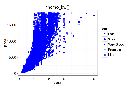
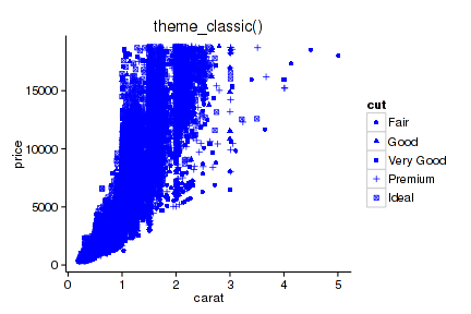
标题文字(字体、字号、颜色)、图形边框和底纹等跟数据无关的一些图形元素的设置都可以归到“主题”这一类。ggplot2提供了4个成套主题:theme_gray(), theme_bw() , theme_minimal() 和 theme_classic()。其中theme_gray()为默认主题,灰背景;后两个是0.9.3版才增加的。
p5 <- p4 + geom_point(color="blue")
p5 + theme_gray() + ggtitle("theme_gray()")
p5 + theme_bw() + ggtitle("theme_bw()")
p5 + theme_minimal() + ggtitle("theme_minimal()")
p5 + theme_classic() + ggtitle("theme_classic()")

2.7 分面 facet:
一页多图,跟图层好像没有直接关系。以后再说。
2.8 标签 labels:
str(p4$labels)
## List of 4
##  $ x     : chr "carat"
##  $ y     : chr "price"
##  $ colour: chr "cut"
##  $ shape : chr "cut"
3 ggplot2做图过程
如果E文水平可以,下载 Hadley Wickham 写的《ggplot2: Elegant Graphics for Data Analysis》一书来看看(到处都有)。理论性太强,太高深,不敢乱说。
4 SessionInfo
sessionInfo()
## R version 3.1.0 (2014-04-10)
## Platform: x86_64-pc-linux-gnu (64-bit)
##
## locale:
##  [1] LC_CTYPE=zh_CN.UTF-8       LC_NUMERIC=C
##  [3] LC_TIME=zh_CN.UTF-8        LC_COLLATE=zh_CN.UTF-8
##  [5] LC_MONETARY=zh_CN.UTF-8    LC_MESSAGES=zh_CN.UTF-8
##  [7] LC_PAPER=zh_CN.UTF-8       LC_NAME=C
##  [9] LC_ADDRESS=C               LC_TELEPHONE=C
## [11] LC_MEASUREMENT=zh_CN.UTF-8 LC_IDENTIFICATION=C
##
## attached base packages:
## [1] tcltk     stats     graphics  grDevices utils     datasets  methods
## [8] base
##
## other attached packages:
## [1] ggplot2_0.9.3.1 zblog_0.1.0     knitr_1.5
##
## loaded via a namespace (and not attached):
##  [1] colorspace_1.2-4 digest_0.6.4     evaluate_0.5.3   formatR_0.10
##  [5] grid_3.1.0       gtable_0.1.2     highr_0.3        labeling_0.2
##  [9] MASS_7.3-31      munsell_0.4.2    plyr_1.8.1       proto_0.3-10
## [13] Rcpp_0.11.1      reshape2_1.2.2   scales_0.2.4     stringr_0.6.2
## [17] tools_3.1.0
原文来自:http://blog.csdn.net/u014801157/article/details/24372503