

当我们进入大数据时代之后,并行运算就十分重要了。什么是大数据呢?引用一句流行语吧:
Big data is hype. Everybody talks about big data; nobody knows exactly what it is.
对于生物学来说,大数据对应的应该是第二代测序技术的兴起。所以我们谈到并行运算,主要是为了处理测序数据。在R中,有许多并行运算的包,HighPerformanceComputing就列举了当前所有的用于并行运算的软件包。为了将它更简单的呈现,我绘制了一张图,以便大家能够对常用的一些并行运算的软件包有一个大约的印象,当人们谈及这些包时,我们会有一个印象。 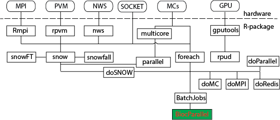 从上图中,可以看到,snow几乎关联了所有的包。但是,因为它很基础,所以很多包对它进行了再一次包装,以达到编程人员即使不了解硬件信息,也可以很轻松地移植并行运算代码的目的。而本文的重点,当然是bioconductor中最新出现的用于parallel运算的包:BiocParallel。它的优势在于它支持了很多bioconductor的类,比如GRanges数据。 下面,我们就通过一个实例来了解如何使用BiocParallel,以及在使用的过程中应该注意些什么。
> ##获取一个大一点的数据
> library(GEOquery)
> setwd("Downloads/")
> getGEOSuppFiles("GSM917672")
[1] "ftp://ftp.ncbi.nlm.nih.gov/geo/samples/GSM917nnn/GSM917672/suppl/"
trying URL 'ftp://ftp.ncbi.nlm.nih.gov/geo/samples/GSM917nnn/GSM917672/suppl//GSM917672_286_+_density.wig.gz'
ftp data connection made, file length 17133766 bytes
opened URL
==================================================
downloaded 16.3 Mb

trying URL 'ftp://ftp.ncbi.nlm.nih.gov/geo/samples/GSM917nnn/GSM917672/suppl//GSM917672_286_-_density.wig.gz'
ftp data connection made, file length 16134038 bytes
opened URL
==================================================
downloaded 15.4 Mb

> setwd("GSM917672/")
> sapply(dir(), gunzip)
$`GSM917672_286_-_density.wig.gz`
character(0)

$`GSM917672_286_+_density.wig.gz`
character(0)
> file <- dir()[1]
> ##将数据读入内存
> s <- file.info(file)$size
> buf <- readChar(file, s, useBytes=TRUE)
> ##将数据按照WIG文件格式说明分割成小段,每一段只包含一段完整的WIG峰值
> buf <- strsplit(buf, "\n", fixed=TRUE, useBytes=TRUE)[[1]]
> infoLine <- grep("Step", buf)
> block <- c(infoLine, length(buf)+1)
> dif <- diff(block)
> block <- rep(infoLine, dif)
> buf <- split(buf, block)
> ##WIG文件的处理
> library(GenomicRanges)
> parser <- function(ele){
+ 	library(GenomicRanges)##在并行运算中,所有的包都需要再次载入,而在非并行运算中只需要载入一次
+ 	firstline <- ele[1]
+ 	firstline <- unlist(strsplit(firstline, "\\s"))
+ 	firstline <- firstline[firstline!=""]
+ 	structure <- firstline[1]
+ 	firstline <- firstline[-1]
+ 	firstline <- do.call(rbind,strsplit(firstline, "=", fixed=TRUE))
+ 	firstline <- firstline[match(c("chrom","span","start","step"),
+ 								 firstline[,1]),]
+ 	wiginfo <- c(structure, firstline[,2])
+ 	names(wiginfo) <- c("structure", "chrom","span","start","step")
+ 	start <- as.numeric(wiginfo["start"])
+ 	end <- start + 1:((length(ele)-1) * as.numeric(wiginfo["step"])) - 1
+ 	start <- c(start, end+1)[1:(length(ele)-1)]
+ 	value <- as.numeric(ele[2:length(ele)])
+ 	GRanges(seqnames=wiginfo["chrom"],
+ 			ranges=IRanges(start, end),
+ 			score=value)
+ }
> ##使用pbapply中pblapply来比较运算速度。因为这个过程中也同样需要输出进度条
> library(pbapply)
> system.time(r1 <- pblapply(buf[1:100], parser))
  |++++++++++++++++++++++++++++++++++++++++++++++++++| 100%
   user  system elapsed
  1.474   0.017   1.512
> system.time(r1 <- pblapply(buf[1:10000], parser))
  |++++++++++++++++++++++++++++++++++++++++++++++++++| 100%
   user  system elapsed
152.830   0.867 157.519
> system.time(r1 <- bplapply(buf[1:50000], parser))
    user   system  elapsed
1247.566    6.536 1257.071
> ##使用BiocParallel来进行运算
> library("BiocParallel")
> library(BatchJobs)
> cluster.functions <- makeClusterFunctionsMulticore()
Setting for worker localhost: ncpus=8
> bpParams <- BatchJobsParam(cluster.functions=cluster.functions)
> system.time(r2 <- bplapply(buf[1:10000], parser, BPPARAM=bpParams))
SubmitJobs |+++++++++++++++++++++++++++++++++++++++++++++++++++++++++++++++++++++++++++++++++| 100% (00:00:00)
Waiting [S:0 R:0 D:10000 E:0] |++++++++++++++++++++++++++++++++++++++++++++++++++++++++++++++++++| 100% (00:00:00)0:16)

   user  system elapsed
  0.425   0.325  10.675
> system.time(r2 <- bplapply(buf[1:10000], parser, BPPARAM=bpParams))
SubmitJobs |+++++++++++++++++++++++++++++++++++++++++++++++++++++++++++++++++++++++++++++++++| 100% (00:00:00)
Waiting [S:0 R:0 D:10000 E:0] |++++++++++++++++++++++++++++++++++++++++++++++++++++++++++++++++++| 100% (00:00:00)0:16)

   user  system elapsed
  7.898   2.351 166.118
> system.time(r2 <- bplapply(buf[1:50000], parser, BPPARAM=bpParams))
SubmitJobs |+++++++++++++++++++++++++++++++++++++++++++++++++++++++++++++++++++++++++++++++++| 100% (00:00:00)
Waiting [S:0 R:0 D:50000 E:0] |++++++++++++++++++++++++++++++++++++++++++++++++++++++++++++++++++| 100% (00:00:00):02:51))

   user  system elapsed
 55.197  11.359 732.627
>
> ##比较运算结果是否一致
> identical(r1, r2)
[1] TRUE
从上面的步骤来看,使用BiocParallel进行运算分为三步走, 第一步,书写线程安全的程序,因为每个内核都会重新启动一个R来进行运算,所以程序的书写必须保证每个全新启动的R都可以正确的在其环境中查找到你所需要的所有变量或者函数。 第二步,设置环境参数。这一步使用makeClusterFunctions相关的函数。示例中我们使用了makeClusterFunctionsMulticore函数,其它还有makeClusterFunctionsInteractive, makeClusterFunctionsLocal, makeClusterFunctionsSSH, makeClusterFunctionsTorque, makeClusterFunctionsSGE, makeClusterFunctionsSLURM,具体可参见:?makeClusterFunctions。 第三步,使用bplapply函数提交运算。 从运算的时效性来看,如果每个单独的线程都只是很小的运算量,使用多核并不一定能节约时间,反而有可能因为等待线程结果而花费更多的时间。所以这种时候,不如使用GPU运算。如果每个单独的线程运算量很大时,使用多核就可以极大的节约时间了。 对R中的并行运算的中文博文,还可以参考:http://algosolo.com/competition/429.html 原文来自:http://pgfe.umassmed.edu/ou/archives/3396