

NicheNet简介
分析原理
大多数细胞通讯的分析方法主要依据公共数据库的配体-受体配对关系,以及配体、受体在细胞亚群的表达情况来推断细胞之间发生了哪些通讯关系,但是配体-受体相互作用如何导致受体细胞内下游靶基因表达变化的分析则很少有方法涉及。NicheNet不同于大多数研究细胞间通讯的方法,它着眼于配体对下游基因调控作用。NicheNet可以预测哪些配体影响另一个细胞中的表达,哪些靶基因受到配体的影响以及哪些信号传导可能参与其中。NicheNet可以促进对感兴趣的细胞间通信过程的功能理解,其分析原理如下:
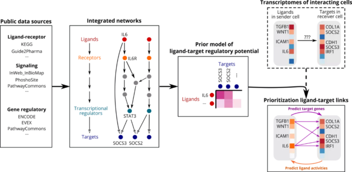
从公共数据库中收集配体-受体配对信息、信号通路、基因调控网络等数据,整合成配体主导的权重配体-靶基因调控模型。然后将可能受到细胞通讯影响的差异基因集输入先验模型,可以计算与这些基因相关的配体的相关性系数。最后挑选根据相关性系数排行靠前的配体,依据先验数据推测与之匹配的受体、靶基因及下游信号网络等信息。
分析流程
确定配体细胞和受体细胞; 确定可能收到配体调控的基因集,可以是case-control的差异基因集,也可以是细胞的signature或其他基因集; 确定一组潜在的配体,它们要在配体细胞中相对高表达(如10%以上的细胞表达),且可以结合受体细胞中的受体(通过先验数据判断); 执行NicheNet配体活性分析,其活性主要通过配体与受体细胞中的差异基因集的相关性进行判断; 推测高活性配体调控的靶基因,以及与配体配对的受体。
安装NicheNet
NicheNet依赖的R包比较多,安装过程可能较长,但是我的安装过程比较顺利,中间没有任何报错。
library(devtools)
install_github("saeyslab/nichenetr")
NicheNet分析实践
数据来源
本文的分析数据和代码来自NicheNet官方分析单细胞数据的教程,https://github.com/saeyslab/nichenetr/blob/master/vignettes/seurat_wrapper.md
演示数据集源自Medaglia et al. 2017 “Spatial Reconstruction of Immune Niches by Combining Photoactivatable Reporters and scRNA-Seq.” Science, December, eaao4277. https://doi.org/10.1126/science.aao4277.
我们将使用Medaglia等人的小鼠NICHE-seq数据,探索淋巴细胞性脉络膜脑膜炎病毒(LCMV)感染之前和之后72小时的腹股沟淋巴结T细胞区域的细胞间通讯。在该数据集中,观察到稳态下的CD8 T细胞与LCMV感染后的CD8 T细胞之间存在差异表达。NicheNet可用于观察淋巴结中的几种免疫细胞群(即单核细胞,树突状细胞,NK细胞,B细胞,CD4 T细胞)如何调节和诱导这些观察到的基因表达变化。
分析准备
library(nichenetr)
library(Seurat)
library(tidyverse)
rm(list=ls())
setwd("~/project/NicheNet")

##读入nichenet先验数据
ligand_target_matrix <- readRDS(url("https://zenodo.org/record/3260758/files/ligand_target_matrix.rds"))
lr_network = readRDS(url("https://zenodo.org/record/3260758/files/lr_network.rds"))
weighted_networks = readRDS(url("https://zenodo.org/record/3260758/files/weighted_networks.rds"))
# weighted_networks列表包含两个数据框,lr_sig是配体-受体权重信号网络,gr是配体-靶基因权重调控网络

##读入单细胞数据
scRNA <- readRDS(url("https://zenodo.org/record/3531889/files/seuratObj.rds"))
scRNA <- UpdateSeuratObject(scRNA)
head(scRNA)
##         nGene nUMI orig.ident aggregate res.0.6 celltype nCount_RNA nFeature_RNA
## W380370   880 1611      LN_SS        SS       1    CD8 T       1607          876
## W380372   541  891      LN_SS        SS       0    CD4 T        885          536
## W380374   742 1229      LN_SS        SS       0    CD4 T       1223          737
## W380378   847 1546      LN_SS        SS       1    CD8 T       1537          838
## W380379   839 1606      LN_SS        SS       0    CD4 T       1603          836
## W380381   517  844      LN_SS        SS       0    CD4 T        840          513
#aggregate是处理条件,SS相当于control,LCMV相当于case。
NicheNet分析
我们希望使用NicheNet预测哪些配体可能影响CD8 T细胞在LCMV感染后的差异表达基因。此例中‘CD8 T cell’是receiver细胞,‘CD4 T’, ‘Treg’, ‘Mono’, ‘NK’, ‘B’ and ‘DC’是sender细胞。
NicheNet提供了一个打包函数nichenet_seuratobj_aggregate,它可以一步完成seurat对象的配体调控网络分析。
Idents(scRNA) <- "celltype"
nichenet_output = nichenet_seuratobj_aggregate(seurat_obj = scRNA,
                                               top_n_ligands = 20,
                                               receiver = "CD8 T",
                                               sender = c("CD4 T","Treg", "Mono", "NK", "B", "DC"),
                                               condition_colname = "aggregate",
                                               condition_oi = "LCMV",
                                               condition_reference = "SS",
                                               ligand_target_matrix = ligand_target_matrix,
                                               lr_network = lr_network,
                                               weighted_networks = weighted_networks,
                                               organism = "mouse")
# top_n_ligands参数指定用于后续分析的高活性配体的数量
NicheNet结果
## 查看配体活性分析结果
# 主要参考pearson指标,bona_fide_ligand=True代表有文献报道的配体-受体,
# bona_fide_ligand=False代表PPI预测未经实验证实的配体-受体。
x <- nichenet_output$ligand_activities
write.csv(x, "ligand_activities.csv", row.names = F)
# 查看top20 ligands
nichenet_output$top_ligands
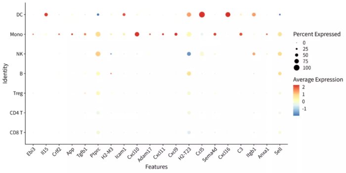
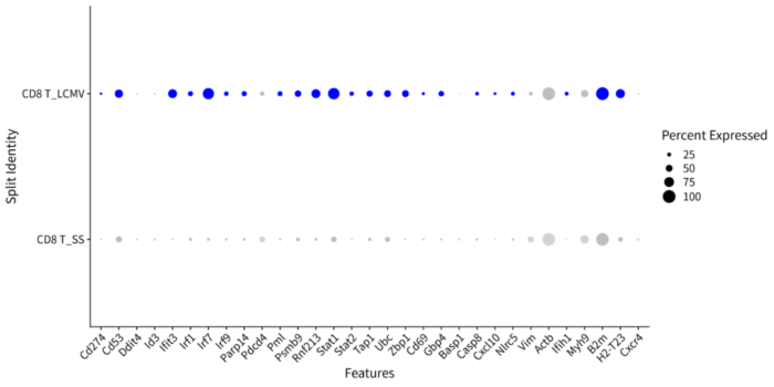
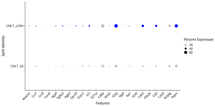
# 查看top20 ligands在各个细胞亚群中表达情况
p = DotPlot(scRNA, features = nichenet_output$top_ligands, cols = "RdYlBu") RotatedAxis()
ggsave("top20_ligands.png", p, width = 12, height = 6)
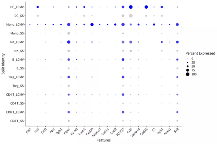
# 按"aggregate"的分类对比配体的表达情况
p = DotPlot(scRNA, features = nichenet_output$top_ligands, split.by = "aggregate") RotatedAxis()
ggsave("top20_ligands_compare.png", p, width = 12, height = 8)
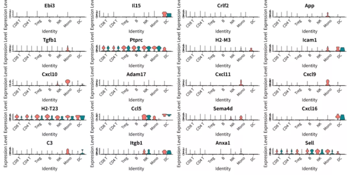
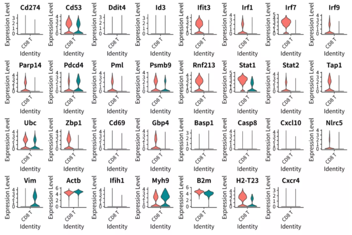
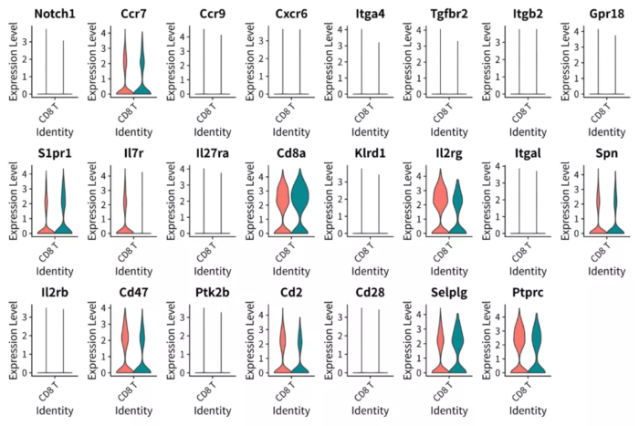
# 用小提琴图对比配体的表达情况
p = VlnPlot(scRNA, features = nichenet_output$top_ligands,
split.by = "aggregate", pt.size = 0, combine = T)
ggsave("VlnPlot_ligands_compare.png", p, width = 12, height = 8)top20_ligands
top20_ligands_compare
VlnPlot_ligands_compare
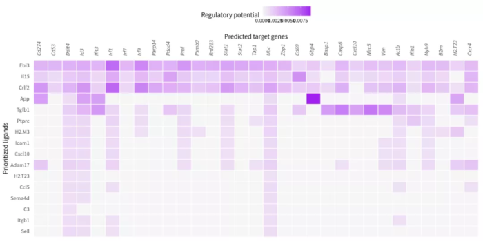
## 查看配体调控靶基因
p = nichenet_output$ligand_target_heatmap
ggsave("Heatmap_ligand-target.png", p, width = 12, height = 6)
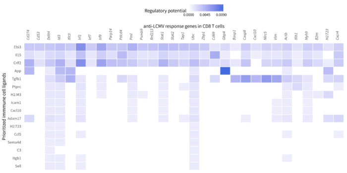
# 更改热图的风格
p = nichenet_output$ligand_target_heatmap
scale_fill_gradient2(low = "whitesmoke", high = "royalblue", breaks = c(0,0.0045,0.009))
xlab("anti-LCMV response genes in CD8 T cells")
ylab("Prioritized immmune cell ligands")
ggsave("Heatmap_ligand-target2.png", p, width = 12, height = 6)
# 查看top配体调控的靶基因及其评分
x <- nichenet_output$ligand_target_matrix
#x2 <- nichenet_output$ligand_target_df
write.csv(x, "ligand_target.csv", row.names = F)
# 查看被配体调控靶基因的表达情况
p = DotPlot(scRNA %>% subset(idents = "CD8 T"),
features = nichenet_output$top_targets,
split.by = "aggregate") RotatedAxis()
ggsave("Targets_Expression_dotplot.png", p, width = 12, height = 6)
p = VlnPlot(scRNA %>% subset(idents = "CD8 T"), features = nichenet_output$top_targets,
split.by = "aggregate", pt.size = 0, combine = T, ncol = 8)
ggsave("Targets_Expression_vlnplot.png", p, width = 12, height = 8)Heatmap_ligand-target
Heatmap_ligand-target2
Targets_Expression_dotplot
Targets_Expression_vlnplot.png
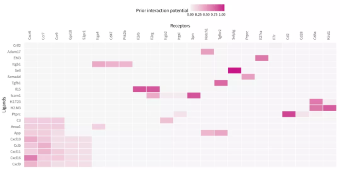
## 查看受体情况
# 查看配体-受体互作
p = nichenet_output$ligand_receptor_heatmap
ggsave("Heatmap_ligand-receptor.png", p, width = 12, height = 6)
x <- nichenet_output$ligand_receptor_matrix
#x <- nichenet_output$ligand_receptor_df
write.csv(x, "ligand_receptor.csv", row.names = F)
# 查看受体表达情况
p = DotPlot(scRNA %>% subset(idents = "CD8 T"),
features = nichenet_output$top_receptors,
split.by = "aggregate") RotatedAxis()
ggsave("Receptors_Expression_dotplot.png", p, width = 12, height = 6)
p = VlnPlot(scRNA %>% subset(idents = "CD8 T"), features = nichenet_output$top_receptors,
split.by = "aggregate", pt.size = 0, combine = T, ncol = 8)
ggsave("Receptors_Expression_vlnplot.png", p, width = 12, height = 8)
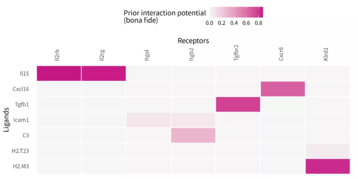
# 有文献报道的配体-受体
# Show ‘bona fide’ ligand-receptor links that are described in the literature and not predicted based on PPI
p = nichenet_output$ligand_receptor_heatmap_bonafide
ggsave("Heatmap_ligand-receptor_bonafide.png", p, width = 8, height = 4)
x <- nichenet_output$ligand_receptor_matrix_bonafide
#x <- nichenet_output$ligand_receptor_df_bonafide
write.csv(x, "ligand_receptor_bonafide.csv", row.names = F)Heatmap_ligand-receptor
Receptors_Expression_dotplot
Receptors_Expression_vlnplot
Heatmap_ligand-receptor_bonafide
如果想深入了解NicheNet,建议大家看看分步完成nichenet分析的教程:https://github.com/saeyslab/nichenetr/blob/master/vignettes/ligand_activity_geneset.md