monocle3简介
monocel3的优势
从UMAP图识别发育轨迹,可以继承Seurat的质控、批次校正和降维分析结果,实现“一张图”展现细胞的聚类、鉴定和轨迹分析结果。 自动对UMAP图分区(partition),可以选择多个起点,轨迹分析算法的逻辑更符合生物学现实。
除了轨迹分析的主要功能,monocle3差异分析方法也有其独到之处,可以做一些与seurat不好实现的分析。
monocel3的安装
先安装一些依赖包,大家安装前可以查看一下这些包是否已经安装过了。
BiocManager::install(c('BiocGenerics', 'DelayedArray', 'DelayedMatrixStats',
                       'limma', 'S4Vectors', 'SingleCellExperiment',
                       'SummarizedExperiment', 'batchelor', 'Matrix.utils'))
然后安装实现umap图分区的包leidenbase,最后安装monole3
install.packages("devtools")
devtools::install_github('cole-trapnell-lab/leidenbase')
devtools::install_github('cole-trapnell-lab/monocle3')
安装有困难的朋友可以使用我的镜像kinesin/rstudio:1.2,下载链接见《kinesin_rstudio的日常升级二》,使用方法见《华为云配置单细胞分析环境及报错处理》。
monocle3分析实践
数据来源
数据来自Immune Landscape of Viral- and Carcinogen-Driven Head and Neck Cancer,数据集GEO编号:GSE139324。建议大家自己下载。原数据集有63个scRNA的数据,都是分选的CD45 免疫细胞。考虑到计算资源问题,挑选了10个样本用于此次演示。
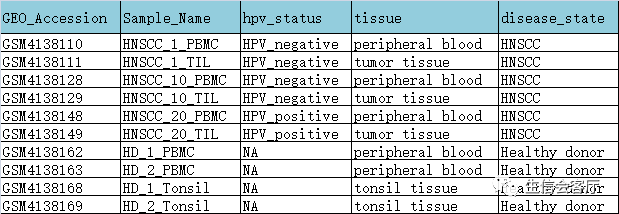
最后用于轨迹分析的细胞是提取的T细胞亚群。
创建seurat对象
library(Seurat)
library(monocle3)
library(tidyverse)
library(patchwork)
rm(list=ls())

##==准备seurat对象列表==##
dir <- dir("GSE139324/")           #GSE139324是存放数据的目录
dir <- paste0("GSE139324/",dir)
sample_name <- c('HNC01PBMC', 'HNC01TIL', 'HNC10PBMC', 'HNC10TIL', 'HNC20PBMC',
                 'HNC20TIL',  'PBMC1', 'PBMC2', 'Tonsil1', 'Tonsil2')
scRNAlist <- list()
for(i in 1:length(dir)){
counts <- Read10X(data.dir = dir[i])
scRNAlist[[i]] <- CreateSeuratObject(counts, project=sample_name[i], min.cells=3, min.features = 200)
scRNAlist[[i]][["percent.mt"]] <- PercentageFeatureSet(scRNAlist[[i]], pattern = "^MT-")
}
scRNA <- merge(scRNAlist[[1]], scRNAlist[2:10])
##提取表达矩阵用于细胞类型鉴定
count <- GetAssayData(scRNA, assay = "RNA", slot = "counts")
saveRDS(count, "count.rds")
利用azimuth鉴定细胞类型
Seurat官网近期推出了在线细胞类型鉴定服务,可以准确鉴定pbmc细胞,建议大家尝试一下。
点击箭头所指的Browse按钮,将上一步保存的count.rds文件上传到网站,网址:http://azimuth.satijalab.org/app/azimuth
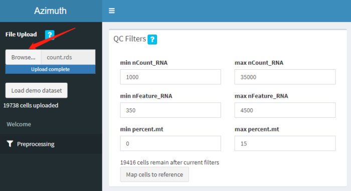
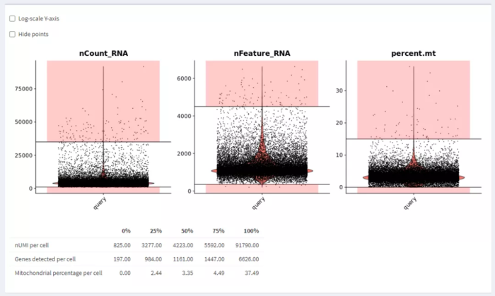
可以按自己的需要设置质控标准,网页会同步展示小提琴图
质控参数确定后,点击Map cells to reference就可以鉴定细胞类型了。

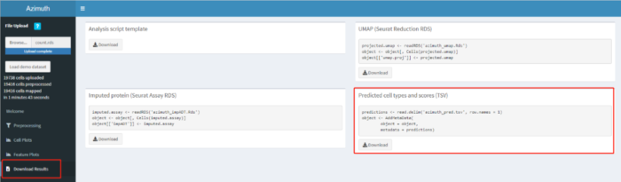
比对成功后,先点击左边红框标注的Download Results,然后下载预测结果
提取T细胞亚群
## 读取azimuth鉴定的结果
pred <- read.delim("azimuth_pred.tsv")
head(pred, 2)
# cell predicted.id predicted.score mapping.score
#1 HNC01PBMC_AAACCTGAGGAGCGTT-1 CD14 Mono 1.0000000 0.8842671
#2 HNC01PBMC_AAACCTGCACGGACAA-1 CD8 TEM 0.3651781 0.8838794
## 提取只含T细胞的子集
pred.T <- subset(pred, pred$predicted.id %in% c('CD4 CTL',
'CD4 Naive',
'CD4 Proliferating',
'CD4 TCM',
'CD4 TEM',
'CD8 Naive',
'CD8 TCM',
'CD8 Proliferating',
'CD8 TEM',
'MAIT',
'Treg',
'dnT',
'gdT'))
scRNAsub <- scRNA[,as.character(pred.T$cell)]
## T细胞子集去除批次效应
scRNAsub <- SCTransform(scRNAsub) %>% RunPCA()
scRNAsub <- RunHarmony(scRNAsub, group.by.vars = "orig.ident",
assay.use = "SCT", max.iter.harmony = 10)
## 降维聚类
ElbowPlot(scRNA, ndims = 50)
pc.num=1:30
scRNAsub <- RunUMAP(scRNAsub, reduction="harmony", dims=pc.num) %>%
FindNeighbors(reduction="harmony", dims=pc.num) %>%
FindClusters(resolution=0.8)
pred.T <- data.frame(pred.T[, c(2,3,4)], row.names = pred.T$cell)
scRNAsub <- AddMetaData(scRNAsub, metadata = pred.T)
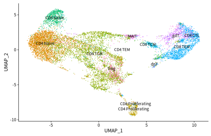
DimPlot(scRNAsub, reduction = "umap", group.by = "predicted.id", label = T) NoLegend()
monocle3轨迹分析
##创建CDS对象并预处理数据
data <- GetAssayData(scRNAsub, assay = 'RNA', slot = 'counts')
cell_metadata <- scRNAsub@meta.data
gene_annotation <- data.frame(gene_short_name = rownames(data))
rownames(gene_annotation) <- rownames(data)
cds <- new_cell_data_set(data,
cell_metadata = cell_metadata,
gene_metadata = gene_annotation)
#preprocess_cds函数相当于seurat中NormalizeData ScaleData RunPCA
cds <- preprocess_cds(cds, num_dim = 50)
#umap降维
cds <- reduce_dimension(cds, preprocess_method = "PCA")
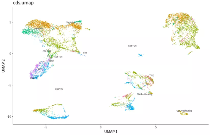
p1 <- plot_cells(cds, reduction_method="UMAP", color_cells_by="celltype") ggtitle('cds.umap')
##从seurat导入整合过的umap坐标
cds.embed <- cds@int_colData$reducedDims$UMAP
int.embed <- Embeddings(scRNAsub, reduction = "umap")
int.embed <- int.embed[rownames(cds.embed),]
cds@int_colData$reducedDims$UMAP <- int.embed
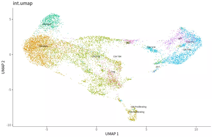
p2 <- plot_cells(cds, reduction_method="UMAP", color_cells_by="celltype") ggtitle('int.umap')
monocle降维的结果
导入整合过的umap坐标后作图
## Monocle3聚类分区
cds <- cluster_cells(cds)
p1 <- plot_cells(cds, show_trajectory_graph = FALSE)   ggtitle("label by clusterID")
p2 <- plot_cells(cds, color_cells_by = "partition", show_trajectory_graph = FALSE)
        ggtitle("label by partitionID")
p = wrap_plots(p1, p2)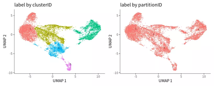
## 识别轨迹
cds <- learn_graph(cds)
p = plot_cells(cds, label_groups_by_cluster = FALSE, label_leaves = FALSE,
               label_branch_points = FALSE)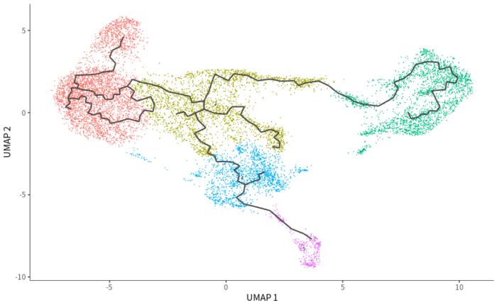
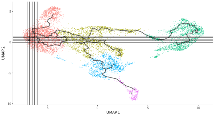
##细胞按拟时排序
# cds <- order_cells(cds) 存在bug,使用辅助线选择root细胞
p geom_vline(xintercept = seq(-7,-6,0.25)) geom_hline(yintercept = seq(0,1,0.25))
embed <- data.frame(Embeddings(scRNAsub, reduction = "umap"))
embed <- subset(embed, UMAP_1 > -6.75 & UMAP_1 < -6.5 & UMAP_2 > 0.24 & UMAP_2 < 0.25)
root.cell <- rownames(embed)
cds <- order_cells(cds, root_cells = root.cell)
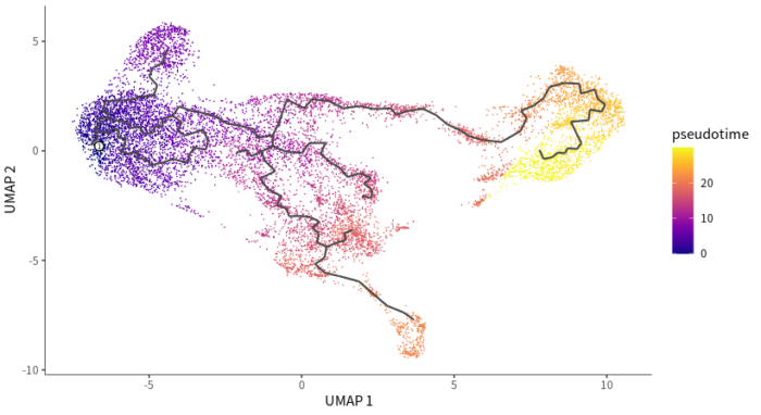
plot_cells(cds, color_cells_by = "pseudotime", label_cell_groups = FALSE,
label_leaves = FALSE, label_branch_points = FALSE)画几条辅助线用于找到root细胞
完成拟时分析的细胞排序结果
monocle3差异分析
##寻找拟时轨迹差异基因
#graph_test分析最重要的结果是莫兰指数(morans_I),其值在-1至1之间,0代表此基因没有
#空间共表达效应,1代表此基因在空间距离相近的细胞中表达值高度相似。
Track_genes <- graph_test(cds, neighbor_graph="principal_graph", cores=10)
#挑选top10画图展示
Track_genes_sig <- Track_genes %>% top_n(n=10, morans_I) %>%
pull(gene_short_name) %>% as.character()
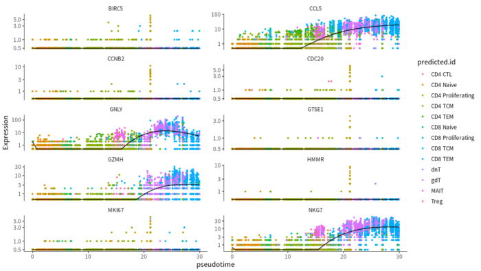
#基因表达趋势图
plot_genes_in_pseudotime(cds[Track_genes_sig,], color_cells_by="predicted.id",
min_expr=0.5, ncol = 2)
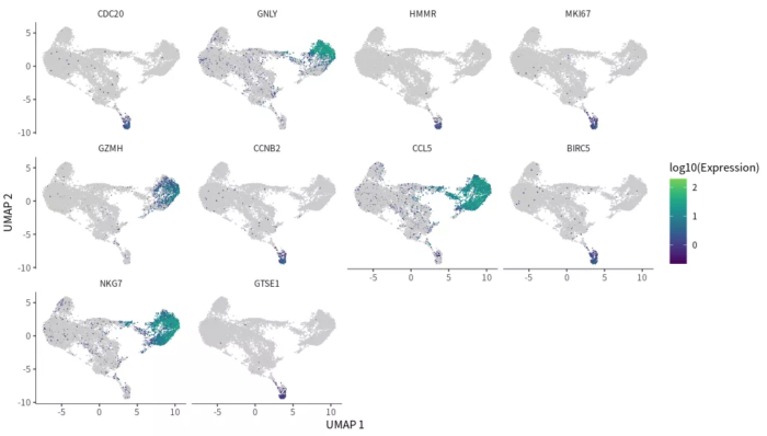
#FeaturePlot图
plot_cells(cds, genes=Track_genes_sig, show_trajectory_graph=FALSE,
label_cell_groups=FALSE, label_leaves=FALSE)
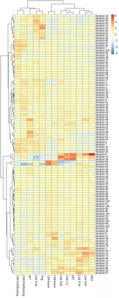
##寻找共表达模块
genelist <- pull(Track_genes, gene_short_name) %>% as.character()
gene_module <- find_gene_modules(cds[genelist,], resolution=1e-2, cores = 10)
cell_group <- tibble::tibble(cell=row.names(colData(cds)),
cell_group=colData(cds)$predicted.id)
agg_mat <- aggregate_gene_expression(cds, gene_module, cell_group)
row.names(agg_mat) <- stringr::str_c("Module ", row.names(agg_mat))
pheatmap::pheatmap(agg_mat, scale="column", clustering_method="ward.D2")基因表达趋势图
FeaturePlot图
共表达模块热图