

写在前面的话:关于细胞通讯的工具有很多,cellchat只是其中一个。网上关于CellChat的解读也很多,我在学习的时候也参考了一些,具体参考列表我都在文中标注了哈。这里只是我在学习细胞通讯和CellChat过程中的学习笔记整理,如果能够对大家有一些帮助就再好不过啦。
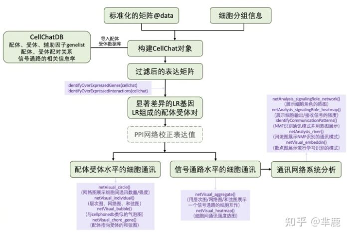
Cell Chat整体分析流程(图片来源:https://www.jianshu.com/p/b3d26ac51c5a)
单个数据集的细胞通讯分析
测试流程:我们就用CellChat来分析一下我们的PBMC数据(有些可视化结果我认为不是特备重要,所以没有实际跑,这里展示就使用教程3中原图代替),看看配受体分析的一般流程。
加载包
# library packages
library(Seurat)
library(dplyr)
library(SeuratData)
library(patchwork) #最强大的拼图包
library(ggplot2)
library(CellChat)
library(ggalluvial)
library(svglite)

rm(list=ls()) #清空所有变量
options(stringsAsFactors = F) #输入数据不自动转换成因子(防止数据格式错误)

getwd()
Part Ⅰ:数据输入&处理、生成CellChat对象
CellChat需要两个输入:
- 一个是细胞的基因表达数据,
- 另一个是细胞标签(即细胞标签)。
对于基因表达数据矩阵,基因应该在带有行名的行中,cell应该在带有名称的列中。CellChat分析的输入是均一化的数据(Seurat@assay$RNA@data)。如果用户提供counts数据,可以用normalizeData函数来均一化。对于细胞的信息,需要一个带有rownames的数据格式作为CellChat的输入。
1.1 加载数据
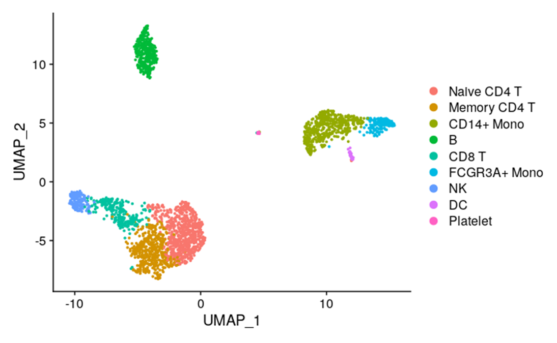
#我们用Seurat给出的pbmc3k.final数据集,大部分的计算已经存在其对象中了:
data_obj <- readRDS("../data/published_data/pbmc3k_final.rds")
DimPlot(data_obj, reduction = "umap")
data_obj$cell_annotations <- Idents(data_obj) # 设置注释slot
data_obj
# An object of class Seurat
# 13714 features across 2638 samples within 1 assay
# Active assay: RNA (13714 features, 2000 variable features)
# 3 dimensional reductions calculated: pca, umap, tsne
pbmc3k.final@commands$FindClusters # 你也看一看作者的其他命令,Seurat是记录其分析过程的。
### 1.2 创建CellChat对象
### 1.3 设置受配体库
```r
CellChatDB <- CellChatDB.human
colnames(CellChatDB$interaction) # 查看一下数据库信息
# 查看数据库具体信息
CellChatDB$interaction[1:4,1:4]
head(CellChatDB$cofactor)
head(CellChatDB$complex)
head(CellChatDB$geneInfo)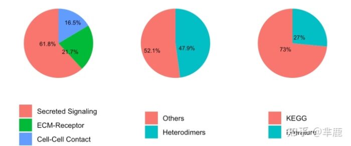
人类中的CellChatDB包含1,939个经过验证的分子相互作用,包括61.8%的旁分泌/自分泌信号相互作用,21.7%的细胞外基质(ECM) - 受体受体相互作用和16.5%的细胞细胞接触相互作用。
CellChatDB记录了许多许多受配体相关的通路信息,不像有的配受体库只有一个基因对。这样,我们就可以更加扎实地把脚落到pathway上面了。在CellChat中,我们还可以先择特定的信息描述细胞间的相互作者,这个可以理解为从特定的侧面来刻画细胞间相互作用, 比用一个大的配体库又精细了许多呢。
# 可以选择的子数据库,用于分析细胞间相互作用
unique(CellChatDB$interaction$annotation)
# [1] "Secreted Signaling" "ECM-Receptor"       "Cell-Cell Contact"

CellChatDB.use <- subsetDB(CellChatDB, search = "Secreted Signaling")
# use Secreted Signaling for cell-cell communication analysis

# Show the structure of the database
dplyr::glimpse(CellChatDB$interaction)llchat@DB <- CellChatDB.use
# set the used database in the object
1.2 预处理表达数据,为细胞通讯分析做准备
cellchat <- subsetData(cellchat) # subset the expression data of signaling genes for saving computation cost
future::plan("multiprocess", workers = 4) # do parallel (可以不设置这一步)
cellchat <- identifyOverExpressedGenes(cellchat) # 相当于suerat中的FindAllMarkers
cellchat <- identifyOverExpressedInteractions(cellchat)
cellchat <- projectData(cellchat, PPI.human)  #储存上一步的结果到cellchat@LR$LRsig
Part Ⅱ:推断配体-受体细胞通讯网络
推断出的配体-受体对的数量取决于计算每个细胞类群平均基因表达的方法。CellChat默认使用的方法是“trimean”,这种方法产生的交互通讯数量较少的,但是有助于我们发现更显著的通讯信息。
2.1 计算通信概率,并推断信号网络
cellchat <- computeCommunProb(cellchat)  #注意这个函数如果你可以用就用,这个是作者的。
# mycomputeCommunProb <-edit(computeCommunProb)  # computeCommunProb内部似乎有一些bug,同一套数据在window10上没事,到了Linux上有报错。发现是computeExpr_antagonist这个函数有问题,(matrix(1, nrow = 1, ncol = length((group)))),中应为(matrix(1, nrow = 1, ncol = length(unique(group))))? 不然矩阵返回的不对。de了它。
# environment(mycomputeCommunProb) <- environment(computeCommunProb)
#cellchat <- mycomputeCommunProb(cellchat)  # 这儿是de过的。
cellchat <- filterCommunication(cellchat, min.cells = 10)


# 可以将推断的结果提取出来
df.net <- subsetCommunication(cellchat)
df.net <- subsetCommunication(cellchat, sources.use = c(1,2), targets.use = c(4,5))#给出从小区组 1 和 2 到小区组 4 和 5 的推断小区间通信。
df.net <- subsetCommunication(cellchat, signaling = c("WNT", "TGFb"))#给出了由信号传导 WNT 和 TGFb 介导的细胞间通讯。
write.csv(df.net, "../output/6_cell_communication/test_cellchat_lr.csv",quote = F,sep = ',')
2.2 计算信号通路水平上的细胞间通讯
CellChat通过汇总与每个信号通路相关的所有配体-受体相互作用的通信概率来计算信号通路水平的通信概率。 注意:推断的每个受配体和么沟通信号通路的细胞通讯网络分别存储在slot "net和“netP”中。
cellchat <- computeCommunProbPathway(cellchat)2.3 计算聚合的细胞间通讯网络
我们可以通过计算链路的数量或汇总通信概率来计算聚合的细胞通信网络。用户还可以通过设置 sources.use
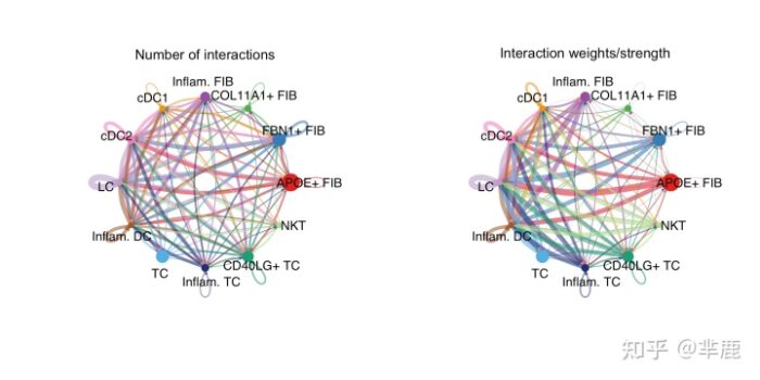
和 targets.use来计算细胞组子集之间的聚合网络``。cellchat <- aggregateNet(cellchat) 我们还可以可视化聚合的细胞间通信网络。例如,使用circle plot显示任意两个细胞组之间的交互次数或总交互强度(权重)。
groupSize <- as.numeric(table(cellchat@idents))
par(mfrow = c(1,2), xpd=TRUE)
netVisual_circle(cellchat@net$count, vertex.weight = groupSize, weight.scale = T, label.edge= F, title.name = "Number of interactions")
netVisual_circle(cellchat@net$weight, vertex.weight = groupSize, weight.scale = T, label.edge= F, title.name = "Interaction weights/strength")
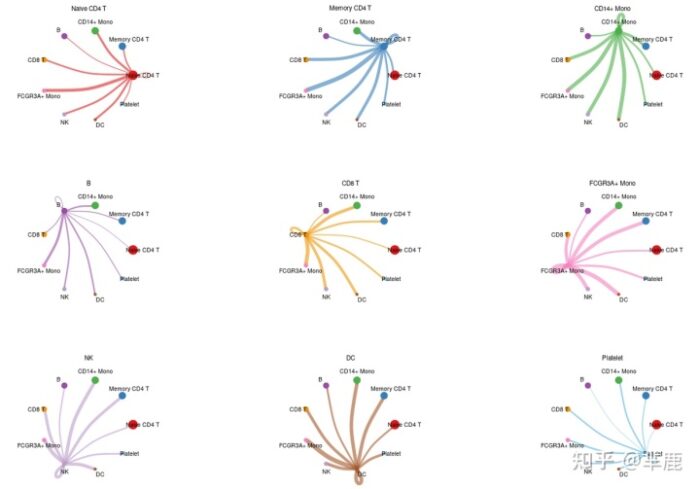
由于细胞间通信网络复杂,我们可以查看各类细胞发出的信号。在这里,我们还控制参数 edge.weight.max
,以便我们可以比较不同网络之间的边缘权重
# 检查每种细胞发出的信号 (每种细胞和其他细胞的互作情况)
mat <- cellchat@net$count
par(mfrow =c(3,3),xpd=T)

for (i in 1:nrow(mat)){
  mat2 <- matrix(0,nrow = nrow(mat),ncol = ncol(mat),dimnames = dimnames(mat))
  mat2[i,] <- mat[i,]
  netVisual_circle(mat2,vertex.weight = groupSize, weight.scale = T, arrow.width = 0.2,
                   arrow.size = 0.1, edge.weight.max = max(mat),title.name = rownames(mat)[i])
}
Part Ⅲ:细胞间通讯网络的可视化
在推断出细胞间通信网络后,CellChat 为进一步的数据探索、分析和可视化提供了各种功能。
- CellChat 提供了几种可视化细胞间通信网络的方法,包括层次图、圆图、弦图和气泡图。
- CellChat 提供了一个易于使用的工具,用于提取和可视化推断网络的高阶信息。例如,它可以方便地预测细胞群的主要信号输入和输出,以及这些群和信号如何协调在一起以实现功能。
- CellChat 可以通过结合社交网络分析、模式识别和流形学习方法,使用集成方法对推断的细胞-细胞通信网络进行定量表征和比较。
3.1 使用层次图、圈图或弦图可视化每个信号通路
# 选择其中一个信号,比如说TGFb
pathways.show <- c("TGFb")
层次图 用户应定义vertex.receiver,这是一个数值向量,将细胞的索引作为层次图左侧的目标(Target)。该分层图由两个部分组成:左侧部分显示对某些感兴趣的细胞(即定义的vertex.receiver)的自分泌和旁分泌信号,右侧部分显示对数据集中剩余细胞的自分泌和旁分泌信号,在层次图中,实心圆和空心圆分别代表源和目标。。因此,层次图提供了一种信息丰富且直观的方式来可视化感兴趣的细胞群之间的自分泌和旁分泌信号通信。例如,在研究成纤维细胞和免疫细胞之间的细胞间通讯时,可以定义vertex.receiver为所有成纤维细胞群。
# Hierarchy plot
# Here we define `vertex.receive` so that the left portion of the hierarchy plot shows signaling to fibroblast and the right portion shows signaling to immune cells
vertex.receiver = seq(1,2,4,6) # a numeric vector.
netVisual_aggregate(cellchat, signaling = pathways.show,  vertex.receiver = vertex.receiver)
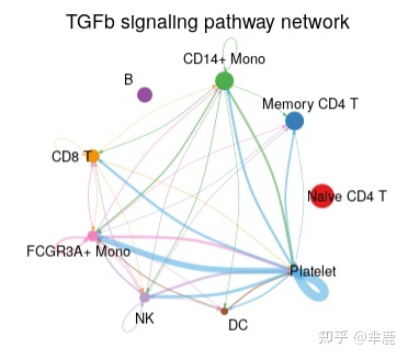
圈图 边缘颜色与信号发出源一致,边缘权重与交互强度成正比。较粗的边缘线表示较强的信号。在Hierarchy plot 和 Circle plot中,圆圈大小与每个细胞类群中的细胞数成正比。
# Circle plot
par(mfrow=c(1,1))
netVisual_aggregate(cellchat, signaling = pathways.show, layout = "circle")
和弦图 CellChatt提供两种功能netVisual_chord_cell, netVisual_chord_gene用于可视化具有不同目的和不同级别的细胞间通信。netVisual_chord_cell 用于可视化不同细胞群间细胞与细胞通讯(和弦图每个扇区都是一个细胞类群),net_Visual_chord_gene用于可视化由多个配受体或信号通路介导的细胞通讯
# Chord diagram
par(mfrow=c(1,1))
netVisual_aggregate(cellchat, signaling = pathways.show, layout = "chord")
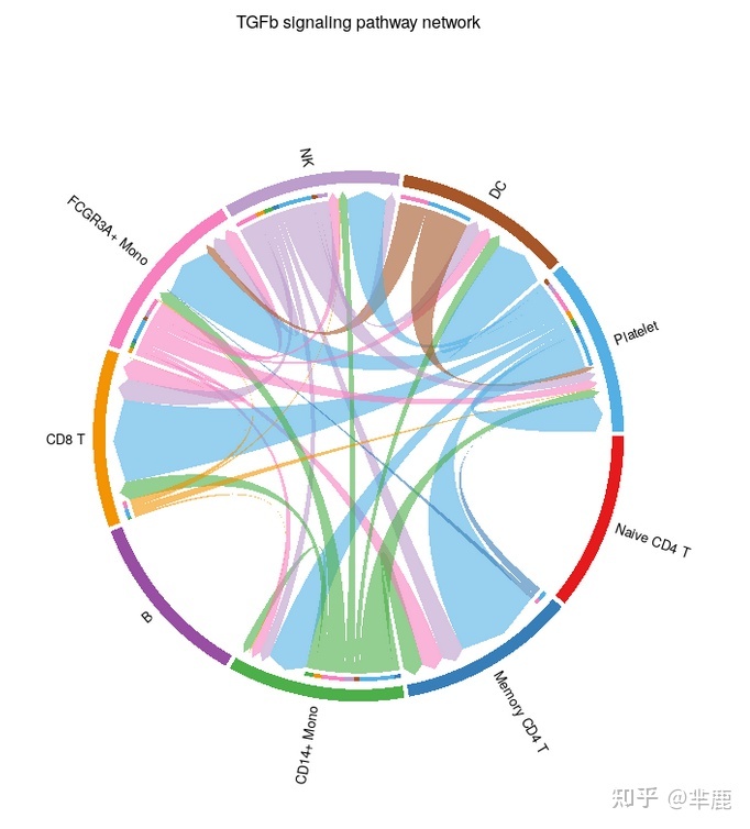
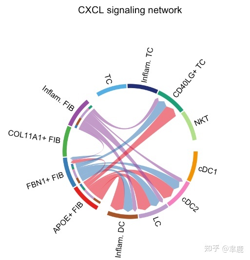
对于和弦图,CellChat 有一个独立的功能netVisual_chord_cell,可以通过调整circlize包中的不同参数来灵活地可视化信令网络。例如,我们可以定义一个命名的字符向量 group 来创建多组和弦图,例如,将细胞簇分组为不同的细胞类型。
# Chord diagram
group.cellType <- c(rep("FIB", 4), rep("DC", 4), rep("TC", 4)) # grouping cell clusters into fibroblast, DC and TC cells
names(group.cellType) <- levels(cellchat@idents)
netVisual_chord_cell(cellchat, signaling = pathways.show, group = group.cellType, title.name = paste0(pathways.show, " signaling network"))
#> Plot the aggregated cell-cell communication network at the signaling pathway level
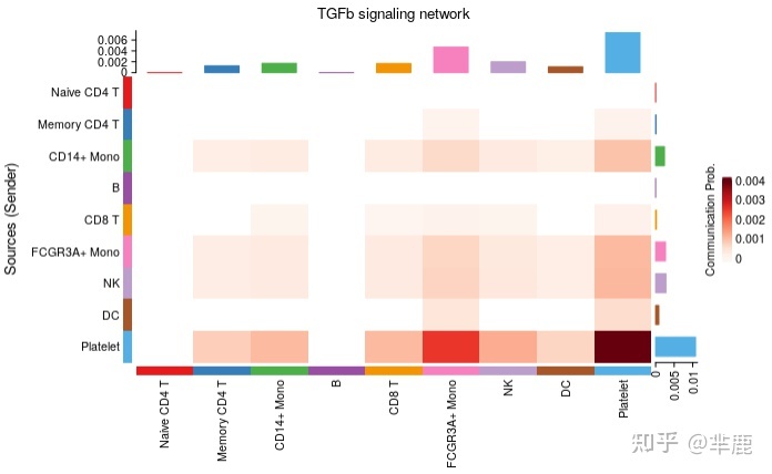
热图
# Heatmap
par(mfrow=c(1,1))
netVisual_heatmap(cellchat, signaling = pathways.show, color.heatmap = "Reds")
#> Do heatmap based on a single object
3.2 计算受配体对整个信号通路的贡献,并可视化单个配体-受体对介导的细胞-细胞通讯
netAnalysis_contribution(cellchat, signaling = pathways.show)
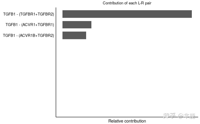
我们还可以可视化由单个配体-受体对介导的细胞间通讯。我们提供了一个函数extractEnrichedLR
来提取给定信号通路的所有重要相互作用(LR 对)和相关信号基因。
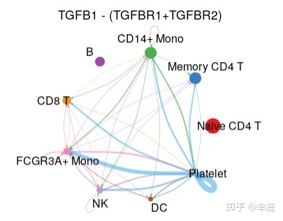
pairLR.TGFb <- extractEnrichedLR(cellchat, signaling = pathways.show, geneLR.return = FALSE)
LR.show <- pairLR.TGFb[1,] # show one ligand-receptor pair
# Hierarchy plot
vertex.receiver = seq(1,2,4,6) # a numeric vector
netVisual_individual(cellchat, signaling = pathways.show,  pairLR.use = LR.show, vertex.receiver = vertex.receiver)
#> [[1]]
# Circle plot
netVisual_individual(cellchat, signaling = pathways.show, pairLR.use = LR.show, layout = "circle")
# Chord diagram
netVisual_individual(cellchat, signaling = pathways.show, pairLR.use = LR.show, layout = "chord")
3.3 自动保存所有推断网络图以便快速探索
在实际使用中,用户可以使用'for ...循环'自动保存所有推断的网络,以便快速探索使用netVisual。
netVisual支持 svg、png和 pdf格式的输出。
# Access all the signaling pathways showing significant communications
pathways.show.all <- cellchat@netP$pathways
# check the order of cell identity to set suitable vertex.receiver
levels(cellchat@idents)
vertex.receiver = seq(1,2,4,6)
for (i in 1:length(pathways.show.all)) {
  # Visualize communication network associated with both signaling pathway and individual L-R pairs
  netVisual(cellchat, signaling = pathways.show.all[i], vertex.receiver = vertex.receiver, layout = "hierarchy")
  # Compute and visualize the contribution of each ligand-receptor pair to the overall signaling pathway
  gg <- netAnalysis_contribution(cellchat, signaling = pathways.show.all[i])
  ggsave(filename=paste0(pathways.show.all[i], "_L-R_contribution.pdf"), plot=gg, width = 3, height = 2, units = 'in', dpi = 300)
}
3.4 可视化由多个受配体或信号通路介导的细胞间通讯
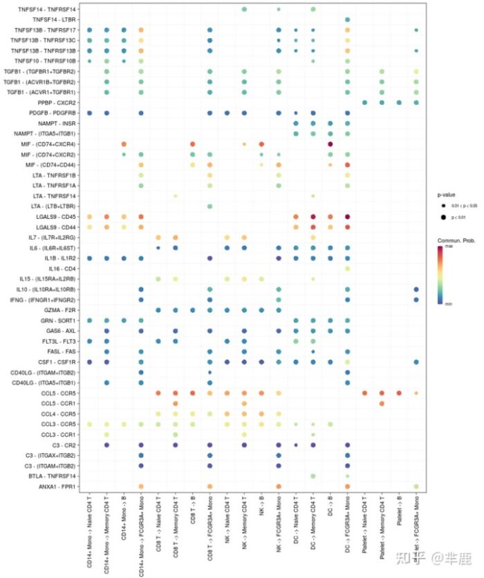
气泡图
# 气泡图(全部配体-受体)

levels(cellcaht@idents)
# show all the significant interactions (L-R pairs)

# 需要制定受体细胞核配体细胞
p=netVisual_bubble(cellchat, sources.use = c(3,5,7,8,9),
                   targets.use = c(1,2,4,6),remove.isolate = FALSE)
p
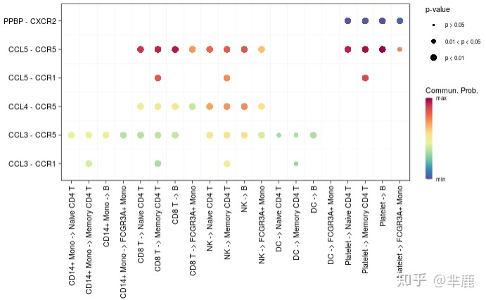
#比如指定CCL和CXCL这两个信号通路
netVisual_bubble(cellchat,sources.use = c(3,5,7,8,9),targets.use = c(1,2,4,6),
                 signaling = c("CCL","CXCL"),remove.isolate = F)
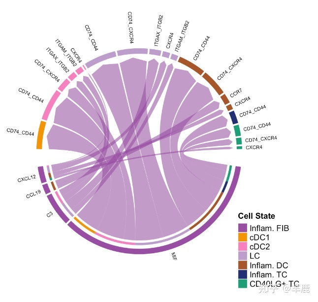
和弦图可视化细胞类群与通讯通路之间的关系 CellChat 与 Bubble plot 类似,提供了netVisual_chord_gene
绘制 Chord 图的功能
- 显示从某些细胞群到其他细胞群的所有相互作用(LR 对或信号通路)。两种特殊情况:一种是显示从一个细胞组发送的所有交互,另一种是显示一个细胞组接收到的所有交互。
- 显示用户输入的交互或用户定义的某些信号通路
# show all the significant interactions (L-R pairs) from some cell groups (defined by 'sources.use') to other cell groups (defined by 'targets.use')
# show all the interactions sending from Inflam.FIB
netVisual_chord_gene(cellchat, sources.use = 4, targets.use = c(5:11), lab.cex = 0.5,legend.pos.y = 30)
# show all the interactions received by Inflam.DC
netVisual_chord_gene(cellchat, sources.use = c(1,2,3,4), targets.use = 8, legend.pos.x = 15)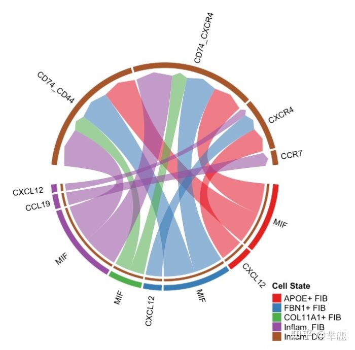
# show all the significant interactions (L-R pairs) associated with certain signaling pathways
netVisual_chord_gene(cellchat, sources.use = c(1,2,3,4), targets.use = c(5:11), signaling = c("CCL","CXCL"),legend.pos.x = 8)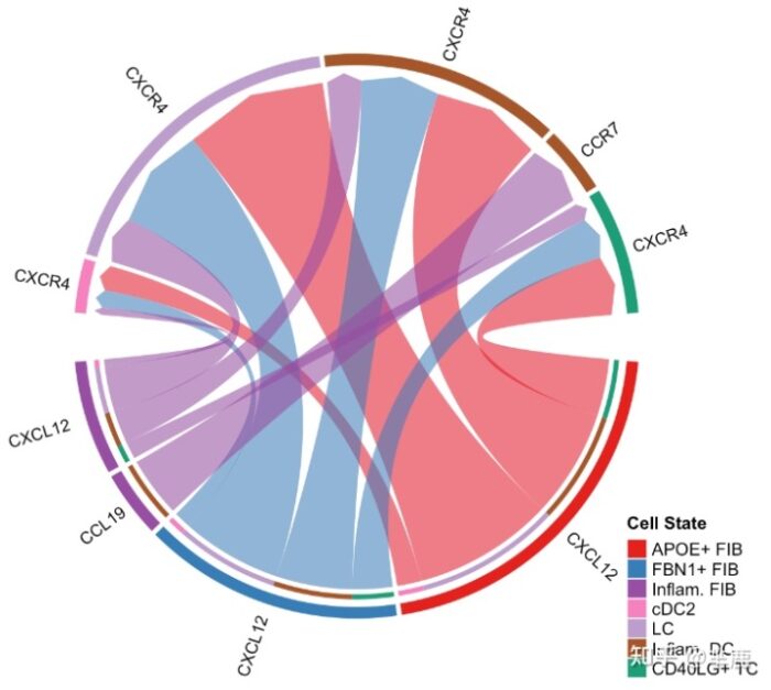
# show all the significant signaling pathways from some cell groups (defined by 'sources.use') to other cell groups (defined by 'targets.use')
netVisual_chord_gene(cellchat, sources.use = c(1,2,3,4), targets.use = c(5:11), slot.name = "netP", legend.pos.x = 10)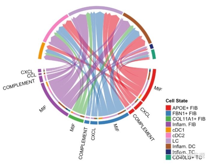
3.5 使用小提琴/点图绘制信号基因表达分布
我们可以使用 Seurat 包装函数绘制与 LR 对或信号通路相关的信号基因的基因表达分布plotGeneExpression。
plotGeneExpression(cellchat, signaling = "CXCL")
#> Registered S3 method overwritten by 'spatstat.geom':
#>   method     from
#>   print.boxx cli
#> Scale for 'y' is already present. Adding another scale for 'y', which will
#> replace the existing scale.
#> Scale for 'y' is already present. Adding another scale for 'y', which will
#> replace the existing scale.
#> Scale for 'y' is already present. Adding another scale for 'y', which will
#> replace the existing scale.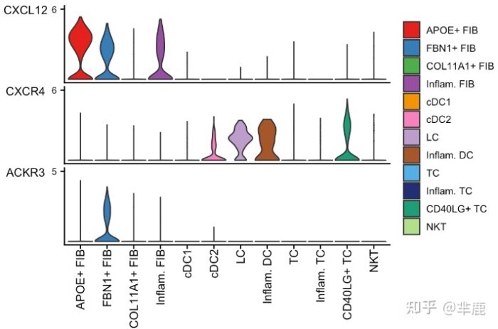
默认情况下,plotGeneExpression仅显示与推断的重要通信相关的信号基因的表达。用户可以通过以下方式显示与一个信号通路相关的所有信号基因的表达。
plotGeneExpression(cellchat, signaling = "CXCL", enriched.only = FALSE)Part Ⅳ:通讯网络系统分析
为了便于解释复杂的细胞间通信网络,CellChat 通过从图论、模式识别和流形学习中抽象出来的方法对网络进行定量测量。
- CellChat可以使用网络分析中的中心性度量来确定给定信号网络内的主要信号源和目标以及中介和影响者
- CellChat可以利用模式识别方法预测特定细胞类型的关键传入和传出信号以及不同细胞类型之间的协调反应。
- CellChat可以通过定义相似性度量并从功能和拓扑角度执行多种学习来对信号通路进行分组。
- CellChat可以通过多个网络的联合流形学习来描绘保守的和特定于上下文的信号通路。
4.1 计算和可视化网络中心性评分
# Compute the network centrality scores
cellchat <- netAnalysis_computeCentrality(cellchat, slot.name = "netP") # the slot 'netP' means the inferred intercellular communication network of signaling pathways
# Visualize the computed centrality scores using heatmap, allowing ready identification of major signaling roles of cell groups
netAnalysis_signalingRole_network(cellchat, signaling = pathways.show, width = 8, height = 2.5, font.size = 10)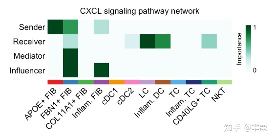
4.2 在二维空间中可视化主要的发送者(源)和接收者(目标)
我们还提供了另一种直观的方法,使用散点图在 2D 空间中可视化主要的发送者(源)和接收者(目标)。
# Signaling role analysis on the aggregated cell-cell communication network from all signaling pathways
gg1 <- netAnalysis_signalingRole_scatter(cellchat)
#> Signaling role analysis on the aggregated cell-cell communication network from all signaling pathways
# Signaling role analysis on the cell-cell communication networks of interest
gg2 <- netAnalysis_signalingRole_scatter(cellchat, signaling = c("CXCL", "CCL"))
#> Signaling role analysis on the cell-cell communication network from user's input
gg1   gg2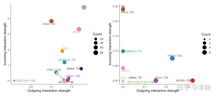
4.3 识别对某些细胞类群的输出和输入信号贡献最大的信号
CellChat还可以回答哪些信号对某些细胞组的传出或传入信号贡献最大的问题。
# Signaling role analysis on the aggregated cell-cell communication network from all signaling pathways
ht1 <- netAnalysis_signalingRole_heatmap(cellchat, pattern = "outgoing")
ht2 <- netAnalysis_signalingRole_heatmap(cellchat, pattern = "incoming")
ht1   ht2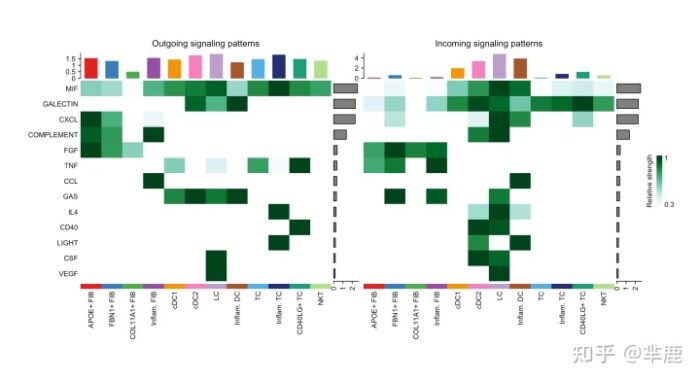
# Signaling role analysis on the cell-cell communication networks of interest
ht <- netAnalysis_signalingRole_heatmap(cellchat, signaling = c("CXCL", "CCL"))
4.4 识别全局通讯模式,探索多种细胞类型和信号通路如何协同工作
除了探索单个通路的详细通信之外,一个重要的问题是多个细胞群和信号通路如何协调发挥作用。CellChat 采用模式识别方法来识别全局通信模式。 识别和可视化分泌细胞的传出通信模式 (pattern) 传出模式揭示了发送细胞(即作为信号源的细胞)如何相互协调,以及它们如何与某些信号通路协调以驱动通信。
#加载通信模式分析所需的包
library(NMF)
#> Loading required package: pkgmaker
#> Loading required package: registry
#> Loading required package: rngtools
#> Loading required package: cluster
#> NMF - BioConductor layer [OK] | Shared memory capabilities [NO: bigmemory] | Cores 15/16
#>   To enable shared memory capabilities, try: install.extras('
#> NMF
#> ')
#>
#> Attaching package: 'NMF'
#> The following objects are masked from 'package:igraph':
#>
#>     algorithm, compare
library(ggalluvial)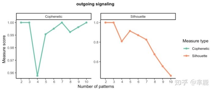
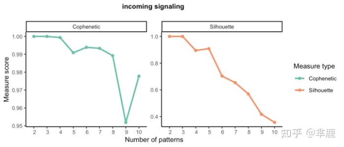
在这里,我们运行selectK以推断模式的数量。
#创建Cellchat 对象
cellchat <- createCellChat(object = data_obj@assays$RNA@data, meta = data_obj@meta.data, group.by = "cell_annotations" )
cellchat

# An object of class CellChat created from a single dataset
# 13714 genes.
# 2638 cells.
当输出模式的数量为 3 时,Cophenetic 和 Silhouette 值都开始突然下降。
nPatterns = 3
cellchat <- identifyCommunicationPatterns(cellchat, pattern = "outgoing", k = nPatterns)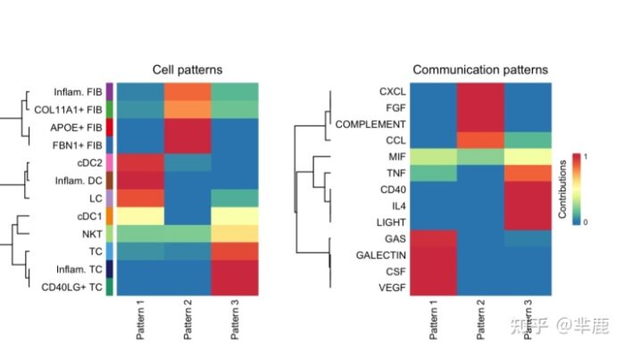
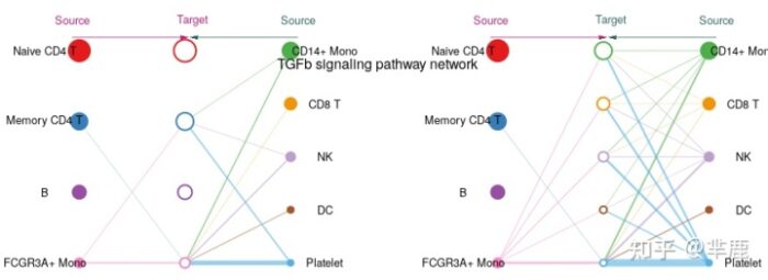
# river plot
netAnalysis_river(cellchat, pattern = "outgoing")
#> Please make sure you have load `library(ggalluvial)` when running this function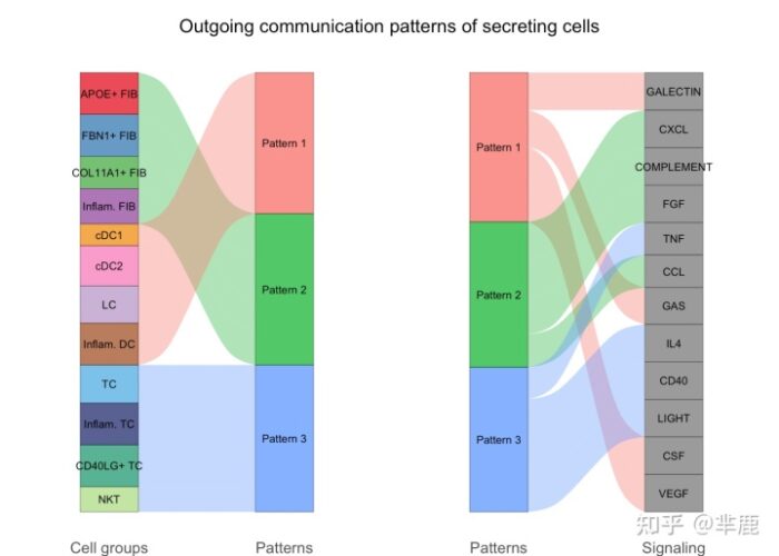
# dot plot
netAnalysis_dot(cellchat, pattern = "outgoing")
识别和可视化目标细胞的传入通信模式
输入模式显示目标细胞(即作为信号接收器的细胞)如何相互协调,以及它们如何与某些信号通路协调以响应输入信号。selectK(cellchat, pattern = "incoming")当传入模式的数量为 4 时,相关值开始下降。
后续同outgoing, 只需要把参数patten 改为 =“incoming”
4.5 信号网络的流行和分类学习分析
CellChat可以量化所有重要悉尼号通路之间的相似性,然后根据她们的通讯网络相似性对她们进行分组。可以根据功能或结构相似性进行分组。(一般功能相似性比较靠谱) 根据功能相似性识别信号组
cellchat <- computeNetSimilarity(cellchat, type = "functional")
cellchat <- netEmbedding(cellchat, type = "functional")
#> Manifold learning of the signaling networks for a single dataset
cellchat <- netClustering(cellchat, type = "functional")
#> Classification learning of the signaling networks for a single dataset
# Visualization in 2D-space
netVisual_embedding(cellchat, type = "functional", label.size = 3.5)

# netVisual_embeddingZoomIn(cellchat, type = "functional", nCol = 2)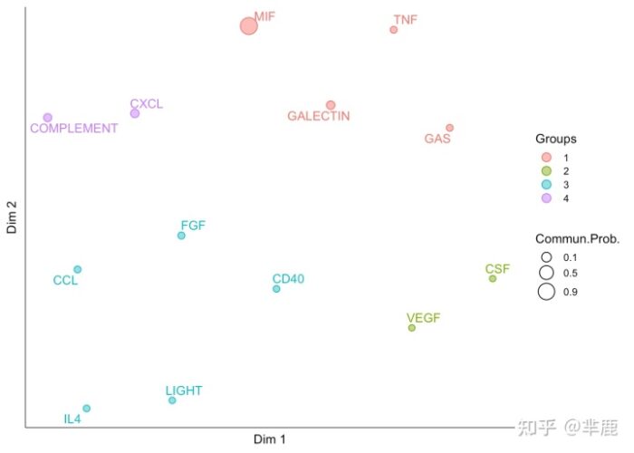
4.6 根据结构相似性识别信号组
cellchat <- computeNetSimilarity(cellchat, type = "structural")
cellchat <- netEmbedding(cellchat, type = "structural")
#> Manifold learning of the signaling networks for a single dataset
cellchat <- netClustering(cellchat, type = "structural")
#> Classification learning of the signaling networks for a single dataset
# Visualization in 2D-space
netVisual_embedding(cellchat, type = "structural", label.size = 3.5)
netVisual_embeddingZoomIn(cellchat, type = "structural", nCol = 2)Part Ⅴ:保存CellChat对象
saveRDS(cellchat, file = "cellchat_humanSkin_LS.rds")

sessionInfo()
#> R version 4.1.2 (2021-11-01)
#> Platform: x86_64-apple-darwin17.0 (64-bit)
#> Running under: macOS Big Sur 10.16
#>
#> Matrix products: default
#> BLAS:   /Library/Frameworks/R.framework/Versions/4.1/Resources/lib/libRblas.0.dylib
#> LAPACK: /Library/Frameworks/R.framework/Versions/4.1/Resources/lib/libRlapack.dylib
#>
#> locale:
#> [1] en_US.UTF-8/en_US.UTF-8/en_US.UTF-8/C/en_US.UTF-8/en_US.UTF-8
#>
#> attached base packages:
#> [1] parallel  stats     graphics  grDevices utils     datasets  methods
#> [8] base
#>
#> other attached packages:
#>  [1] doParallel_1.0.16   iterators_1.0.13    foreach_1.5.1
#>  [4] ggalluvial_0.12.3   NMF_0.23.0          cluster_2.1.2
#>  [7] rngtools_1.5.2      pkgmaker_0.32.2     registry_0.5-1
#> [10] patchwork_1.1.1     CellChat_1.4.0      Biobase_2.54.0
#> [13] BiocGenerics_0.40.0 ggplot2_3.3.5       igraph_1.2.10
#> [16] dplyr_1.0.7
#>
#> loaded via a namespace (and not attached):
#>   [1] backports_1.4.1       circlize_0.4.13       systemfonts_1.0.2
#>   [4] plyr_1.8.6            lazyeval_0.2.2        splines_4.1.2
#>   [7] listenv_0.8.0         scattermore_0.7       gridBase_0.4-7
#>  [10] digest_0.6.29         htmltools_0.5.2       fansi_0.5.0
#>  [13] magrittr_2.0.1        tensor_1.5            ROCR_1.0-11
#>  [16] sna_2.6               ComplexHeatmap_2.10.0 globals_0.14.0
#>  [19] matrixStats_0.61.0    svglite_2.0.0         spatstat.sparse_2.1-0
#>  [22] colorspace_2.0-2      ggrepel_0.9.1         xfun_0.29
#>  [25] crayon_1.4.2          jsonlite_1.7.2        spatstat.data_2.1-2
#>  [28] survival_3.2-13       zoo_1.8-9             glue_1.6.0
#>  [31] polyclip_1.10-0       gtable_0.3.0          leiden_0.3.9
#>  [34] GetoptLong_1.0.5      car_3.0-12            future.apply_1.8.1
#>  [37] shape_1.4.6           abind_1.4-5           scales_1.1.1
#>  [40] DBI_1.1.2             rstatix_0.7.0         miniUI_0.1.1.1
#>  [43] Rcpp_1.0.7            viridisLite_0.4.0     xtable_1.8-4
#>  [46] clue_0.3-60           spatstat.core_2.3-2   reticulate_1.22
#>  [49] stats4_4.1.2          htmlwidgets_1.5.4     httr_1.4.2
#>  [52] FNN_1.1.3             RColorBrewer_1.1-2    ellipsis_0.3.2
#>  [55] Seurat_4.0.6          ica_1.0-2             pkgconfig_2.0.3
#>  [58] farver_2.1.0          uwot_0.1.11           deldir_1.0-6
#>  [61] sass_0.4.0            here_1.0.1            utf8_1.2.2
#>  [64] later_1.3.0           tidyselect_1.1.1      labeling_0.4.2
#>  [67] rlang_0.4.12          reshape2_1.4.4        munsell_0.5.0
#>  [70] tools_4.1.2           cli_3.1.0             generics_0.1.1
#>  [73] statnet.common_4.5.0  broom_0.7.10          ggridges_0.5.3
#>  [76] evaluate_0.14         stringr_1.4.0         fastmap_1.1.0
#>  [79] goftest_1.2-3         yaml_2.2.1            knitr_1.37
#>  [82] fitdistrplus_1.1-6    purrr_0.3.4           RANN_2.6.1
#>  [85] nlme_3.1-153          pbapply_1.5-0         future_1.23.0
#>  [88] mime_0.12             compiler_4.1.2        rstudioapi_0.13
#>  [91] plotly_4.10.0         png_0.1-7             ggsignif_0.6.3
#>  [94] spatstat.utils_2.3-0  tibble_3.1.6          bslib_0.3.1
#>  [97] stringi_1.7.6         highr_0.9             RSpectra_0.16-0
#> [100] forcats_0.5.1         lattice_0.20-45       Matrix_1.3-4
#> [103] vctrs_0.3.8           pillar_1.6.4          lifecycle_1.0.1
#> [106] spatstat.geom_2.3-1   lmtest_0.9-39         jquerylib_0.1.4
#> [109] GlobalOptions_0.1.2   RcppAnnoy_0.0.19      data.table_1.14.2
#> [112] cowplot_1.1.1         irlba_2.3.5           httpuv_1.6.4
#> [115] R6_2.5.1              promises_1.2.0.1      network_1.17.1
#> [118] gridExtra_2.3         KernSmooth_2.23-20    IRanges_2.28.0
#> [121] parallelly_1.30.0     codetools_0.2-18      MASS_7.3-54
#> [124] assertthat_0.2.1      rprojroot_2.0.2       rjson_0.2.20
#> [127] withr_2.4.3           SeuratObject_4.0.4    sctransform_0.3.2
#> [130] S4Vectors_0.32.3      mgcv_1.8-38           rpart_4.1-15
#> [133] grid_4.1.2            tidyr_1.1.4           coda_0.19-4
#> [136] rmarkdown_2.11        carData_3.0-4         Rtsne_0.15
#> [139] ggpubr_0.4.0          shiny_1.7.1