WGCNA加权基因共表达网络分析

序章

这个工具现在很火，高分文章用到很多。

• 加权基因共表达网络分析(WGCNA，Weighted gene co-expression network analysis)
• WGCNA能够从复杂数据中（N多分组）快速地提取出与样本特征相关的基因共表达模块，以供后续分析。简单地说，它通过计算基因之间的表达相关性，将具有表达相关性的基因聚类到一个模块中，然后再分析模块与样本特征（包括临床特征、手术方式、治疗方法等等）之间的相关性，WGCNA搭建了一座样本特征与基因表达变化之间的桥梁。

1. 材料准备

• 文件下载

链接：http://pan.baidu.com/s/1bpvu9Dt
密码：w7g4

• 软件安装

source("http://bioconductor.org/biocLite.R"); 
biocLite("WGCNA")

2. 实战

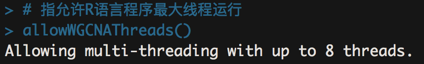
# 导入数据
library(WGCNA)
options(stringsAsFactors = FALSE)
# 指允许R语言程序最大线程运行
allowWGCNAThreads()

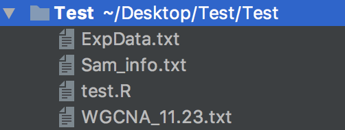
# 设置工作目录路径，R脚本语言和文件夹在同一个目录下
setwd("/Users/chengkai/Desktop/Test")
samples=read.csv('Sam_info.txt',sep = 't',row.names = 1)
expro=read.csv('ExpData.txt',sep = 't',row.names = 1)
dim(expro)

##筛选方差前25%的基因##
m.vars=apply(expro,1,var)
expro.upper=expro[which(m.vars>quantile(m.vars, probs = seq(0, 1, 0.25))[4]),]
dim(expro.upper)
datExpr=as.data.frame(t(expro.upper));
nGenes = ncol(datExpr)
nSamples = nrow(datExpr)

• 上一步是为了减少运算量，因为一个测序数据可能会有好几万个探针，而可能其中很多基因在各个样本中的表达情况并没有什么太大变化，为了减少运算量，这里我们筛选方差前25%的基因。

##样本聚类检查离群值##
gsg = goodSamplesGenes(datExpr, verbose = 3);
gsg$allOK
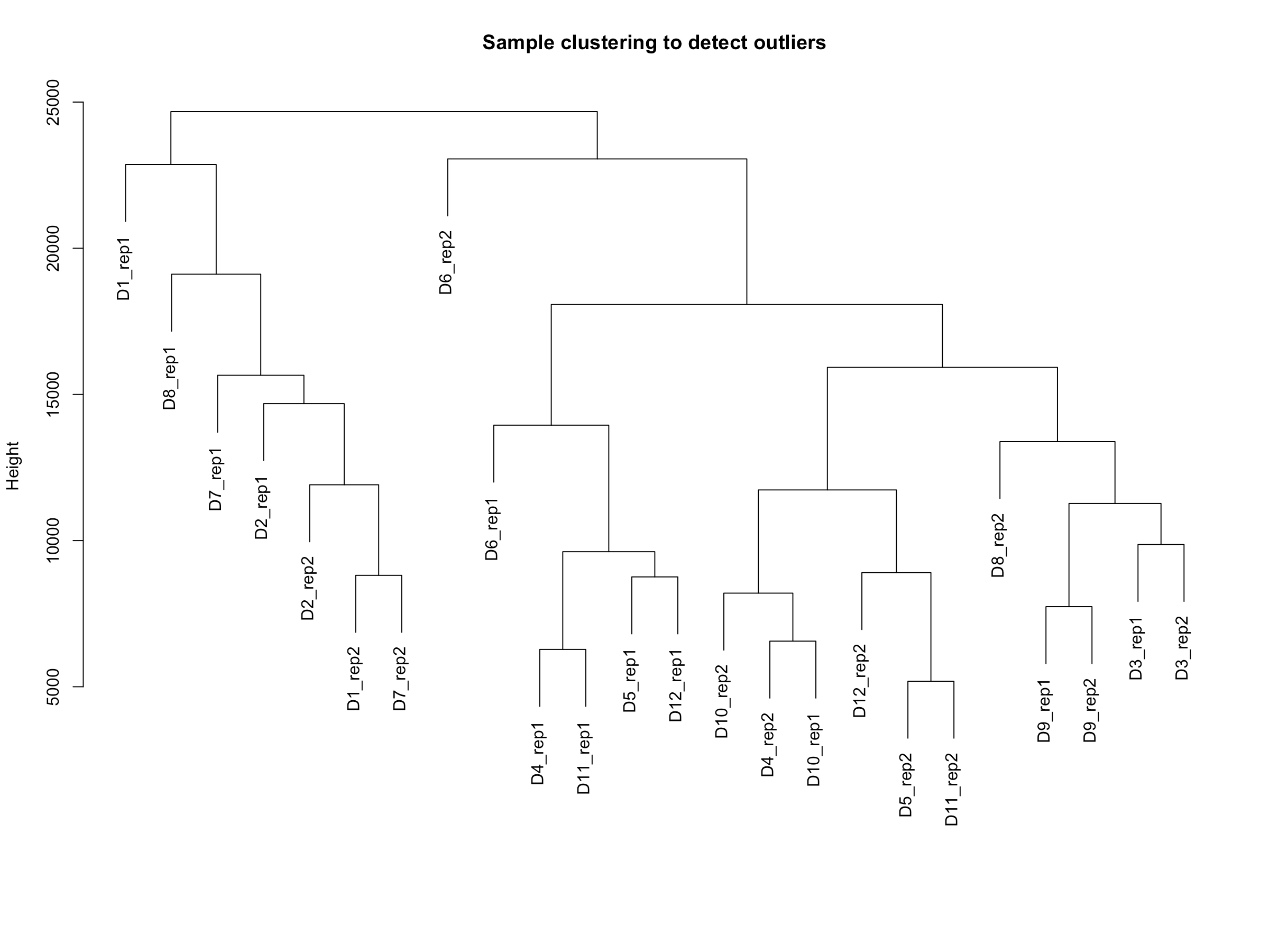
sampleTree = hclust(dist(datExpr), method = "average")
plot(sampleTree, main = "Sample clustering to detect outliers"
     , sub="", xlab="")
save(datExpr, file = "FPKM-01-dataInput.RData")

• 从结果上来，我们分析的样本没啥离群值，所以代码里说不作处理。
• 一个离群值的案例
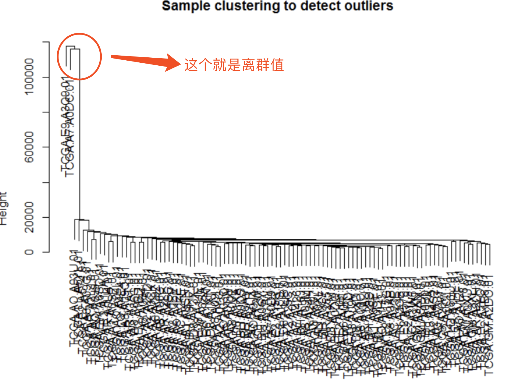
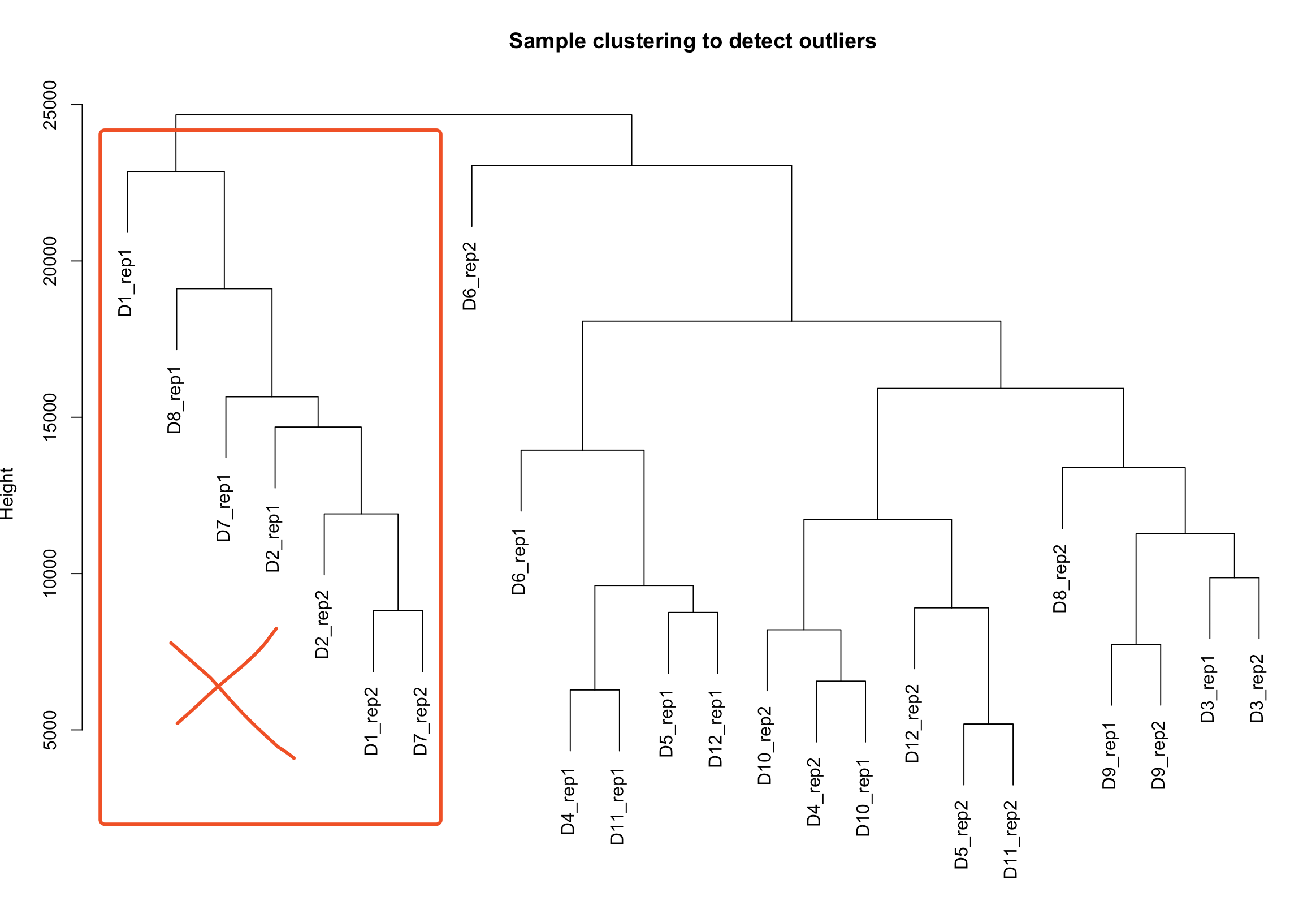
• 如果需要去除离群样本，则执行下列代码，其中cutHeight=多少就看你自己了。

clust = cutreeStatic(sampleTree, cutHeight = 20000, minSize = 10)
table(clust)
keepSamples = (clust==1)
datExpr = datExpr[keepSamples, ]
nGenes = ncol(datExpr)
nSamples = nrow(datExpr)
save(datExpr, file = "FPKM-01-dataInput.RData")

• 执行上述代码的话，就会去掉8个样本

##软阈值筛选##
powers = c(seq(1,10,by = 1), seq(12, 20, by = 2))
sft = pickSoftThreshold(datExpr, powerVector = powers, verbose = 5)
par(mfrow = c(1,2));
cex1 = 0.9;
plot(sft$fitIndices[,1], -sign(sft$fitIndices[,3])*sft$fitIndices[,2],
     xlab="Soft Threshold (power)",ylab="Scale Free Topology Model Fit,signed R^2",type="n",
     main = paste("Scale independence"));
text(sft$fitIndices[,1], -sign(sft$fitIndices[,3])*sft$fitIndices[,2],
     labels=powers,cex=cex1,col="red");
abline(h=0.90,col="red")
plot(sft$fitIndices[,1], sft$fitIndices[,5],
     xlab="Soft Threshold (power)",ylab="Mean Connectivity", type="n",
     main = paste("Mean connectivity"))
text(sft$fitIndices[,1], sft$fitIndices[,5], labels=powers, cex=cex1,col="red")

• 软阈值是WGCNA的算法中非常重要的一个环节，简单的说硬阈值是一种一刀切的算法，比如高考分数>500分能上一本，低于500就不行，软阈值的话切起来比较柔和一些，会考虑你学校怎么样，平时成绩怎么样之类。

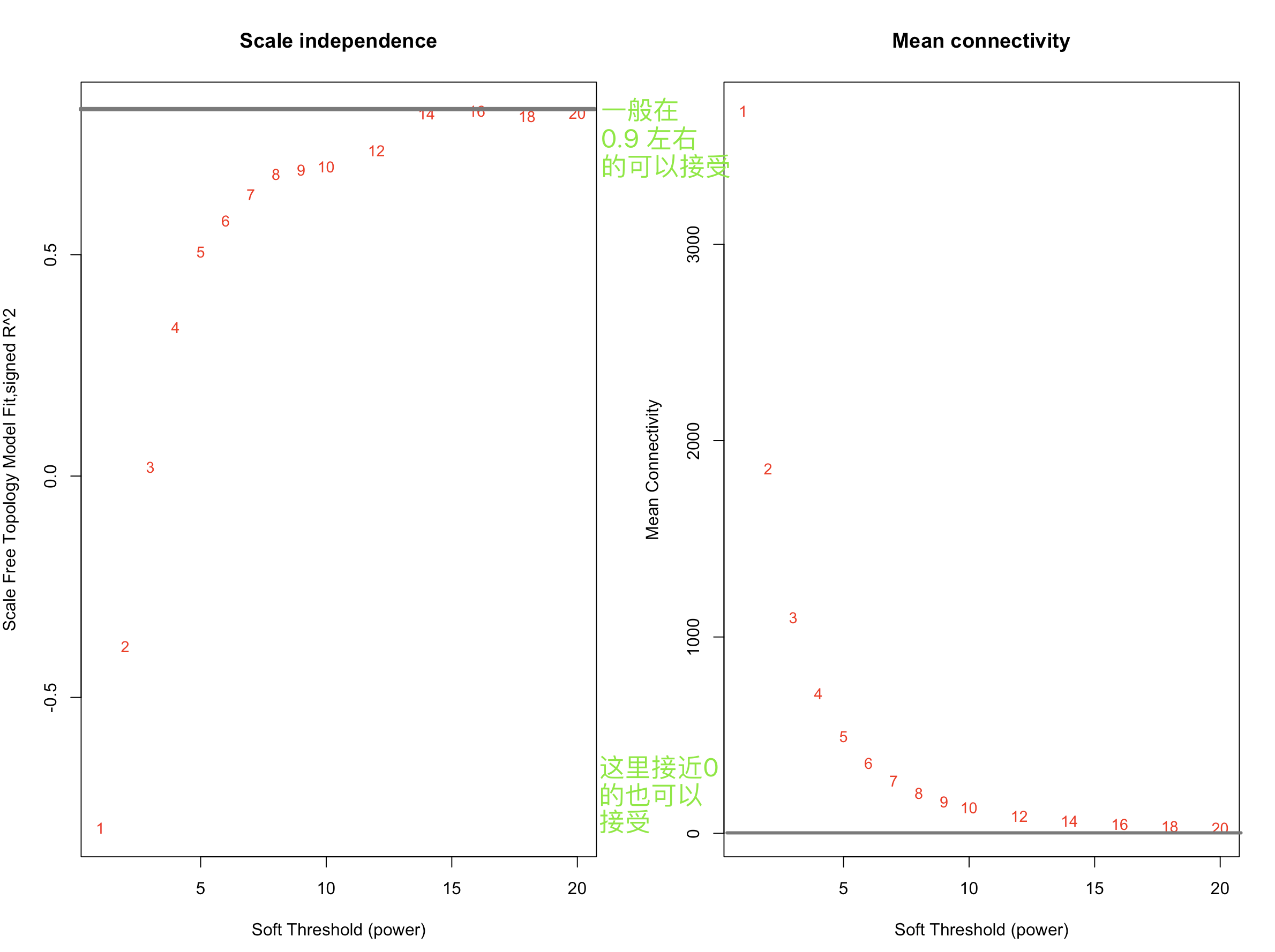
# 运行下列代码，让程序推荐你一个power, 数据质量太差啦，程序给了我"NA",自己设定power=14
> sft$powerEstimate
[1] NA

##一步法网络构建：One-step network construction and module detection##
net = blockwiseModules(datExpr, power = 14, maxBlockSize = 6000,
                       TOMType = "unsigned", minModuleSize = 30,
                       reassignThreshold = 0, mergeCutHeight = 0.25,
                       numericLabels = TRUE, pamRespectsDendro = FALSE,
                       saveTOMs = TRUE,
                       saveTOMFileBase = "AS-green-FPKM-TOM",
                       verbose = 3)
table(net$colors)
sft$powerEstimate

• 结果跑出来如下图
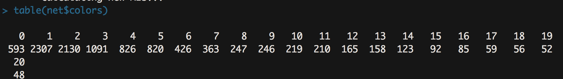
• 结果是每个模块中包含的基因数量。一般来说，结果包含十几个到二十几个模块是比较正常的，此外一个模块中的基因数量不宜过多，像我们这个结果里模块1的基因数量达到了2307，这个就有点太多了，主要是因为我们powers=14，软阈值太低了导致的。所以说上述软阈值的筛选可以对我们的模块分析起到微调的作用。

##绘画结果展示### open a graphics window
#sizeGrWindow(12, 9)
# Convert labels to colors for plotting
mergedColors = labels2colors(net$colors)
# Plot the dendrogram and the module colors underneath
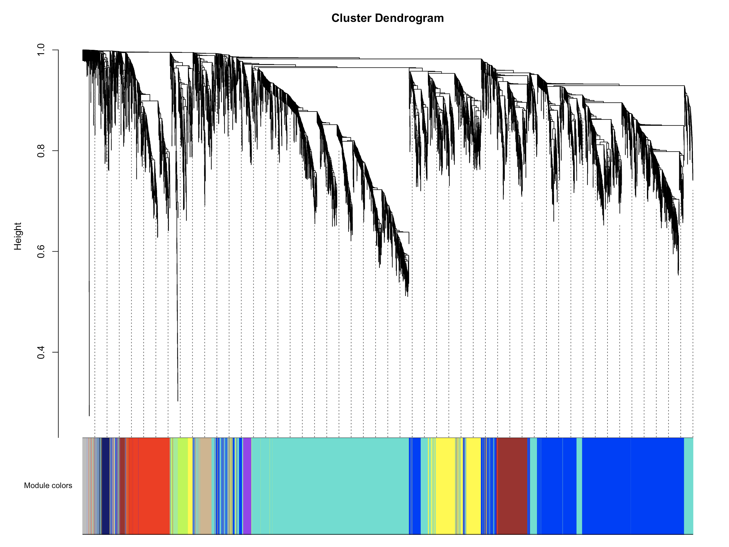
plotDendroAndColors(net$dendrograms[[1]], mergedColors[net$blockGenes[[1]]],"Module colors",
                    dendroLabels = FALSE, hang = 0.03,
                    addGuide = TRUE, guideHang = 0.05)

• 由于我们的软阈值比较低，所以这一结果中几乎没有grey模块，grey模块中的基因是共表达分析时没有被接受的基因，可以理解为一群散兵游勇。当然如果分析结果中grey模块中的基因数量比较多也是不太好的，表示样本中的基因共表达趋势不明显，不同特征的样本之间差异性不大，或者组内基因表达一致性比较差。

##结果保存###
moduleLabels = net$colors
moduleColors = labels2colors(net$colors)
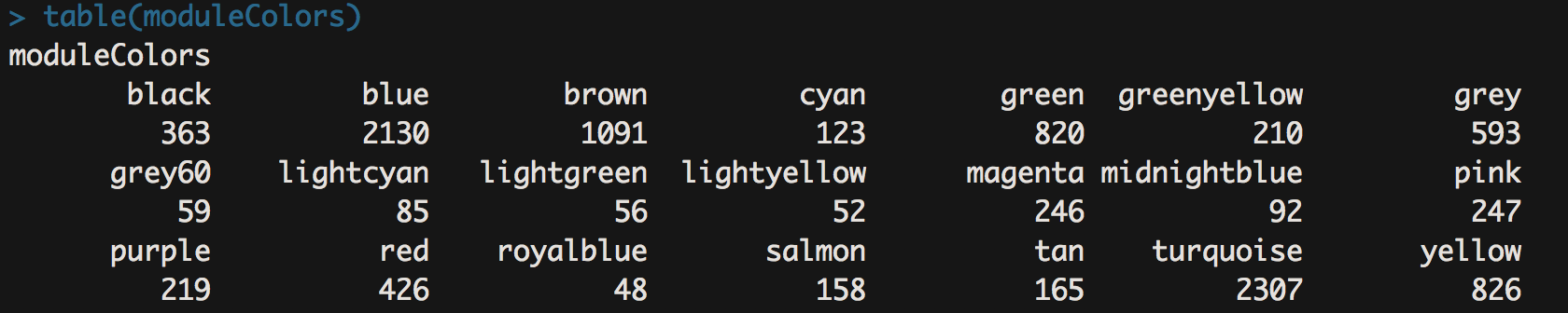
table(moduleColors)
MEs = net$MEs;
geneTree = net$dendrograms[[1]];
save(MEs, moduleLabels, moduleColors, geneTree,
     file = "AS-green-FPKM-02-networkConstruction-auto.RData")

• 这一步就是保存上面跑出来的结果了，同时哪个模块有多少基因一目了然。

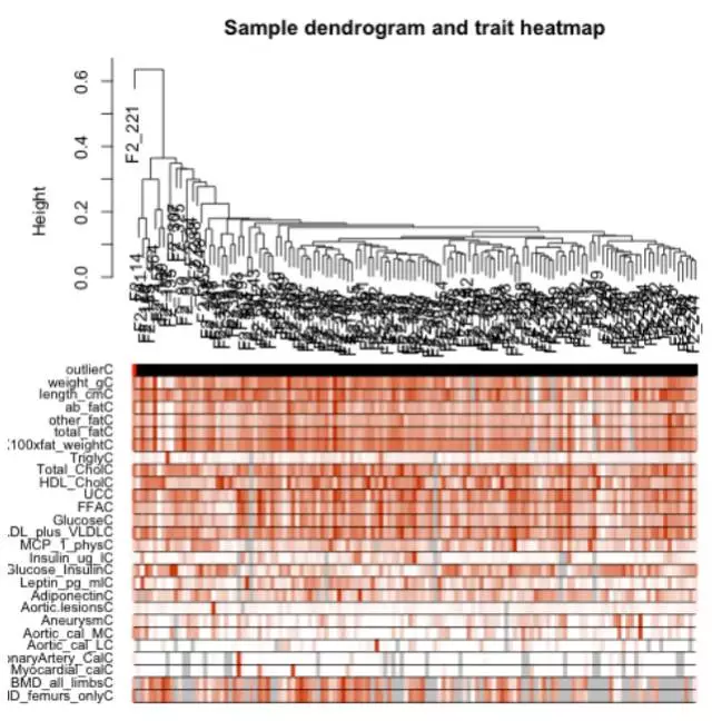
##表型与模块相关性##
moduleLabelsAutomatic = net$colors
moduleColorsAutomatic = labels2colors(moduleLabelsAutomatic)
moduleColorsWW = moduleColorsAutomatic
MEs0 = moduleEigengenes(datExpr, moduleColorsWW)$eigengenes
MEsWW = orderMEs(MEs0)
modTraitCor = cor(MEsWW, samples, use = "p")
colnames(MEsWW)
modlues=MEsWW

modTraitP = corPvalueStudent(modTraitCor, nSamples)
textMatrix = paste(signif(modTraitCor, 2), "n(", signif(modTraitP, 1), ")", sep = "")
dim(textMatrix) = dim(modTraitCor)
labeledHeatmap(Matrix = modTraitCor, xLabels = colnames(samples), yLabels = names(MEsWW), cex.lab = 0.9,  yColorWidth=0.01, 
               xColorWidth = 0.03,
               ySymbols = colnames(modlues), colorLabels = FALSE, colors = blueWhiteRed(50), 
               textMatrix = textMatrix, setStdMargins = FALSE, cex.text = 0.5, zlim = c(-1,1)
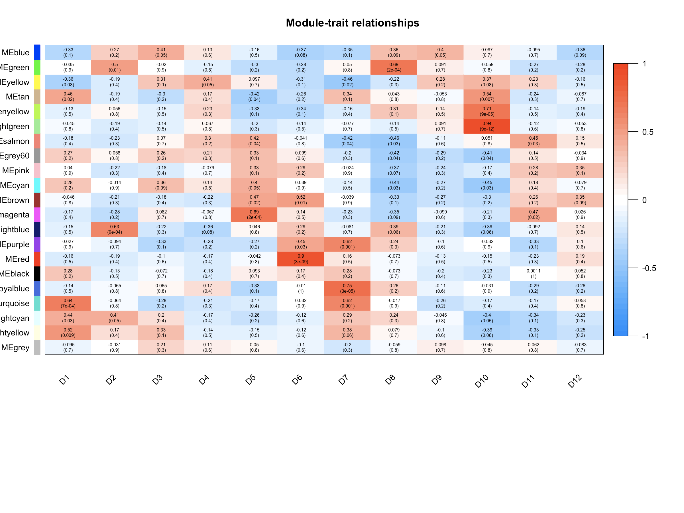
               , main = paste("Module-trait relationships"))

• cex.lab可以更改X轴Y轴label字体的大小，cex.text可以更改热图中字体的大小，colors可以改变颜色。
• 样本特征和共表达模块的相关性热图中，grey模块中的相关性应该很小，如果你与样本特征相关性最显著的模块是grey模块，那肯定是有问题的，毕竟grey模块中的基因是一群散兵游勇，它们的表达在各个样本中杂乱无章，根本说明不了问题。

###导出网络到Cytoscape#### Recalculate topological overlap if needed
TOM = TOMsimilarityFromExpr(datExpr, power = 14);
# Read in the annotation file# annot = read.csv(file = "GeneAnnotation.csv");
# Select modules需要修改，选择需要导出的模块颜色
modules = c("lightgreen");
# Select module probes选择模块探测

probes = names(datExpr)
inModule = is.finite(match(moduleColors, modules));
modProbes = probes[inModule];
#modGenes = annot$gene_symbol[match(modProbes, annot$substanceBXH)];
# Select the corresponding Topological Overlap
modTOM = TOM[inModule, inModule];
dimnames(modTOM) = list(modProbes, modProbes)
# Export the network into edge and node list files Cytoscape can read
cyt = exportNetworkToCytoscape(modTOM,
                               edgeFile = paste("AS-green-FPKM-One-step-CytoscapeInput-edges-", paste(modules, collapse="-"), ".txt", sep=""),
                               nodeFile = paste("AS-green-FPKM-One-step-CytoscapeInput-nodes-", paste(modules, collapse="-"), ".txt", sep=""),
                               weighted = TRUE,
                               threshold = 0.02,
                               nodeNames = modProbes,                               
#altNodeNames = modGenes,
                               nodeAttr = moduleColors[inModule]);

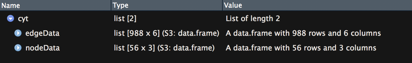
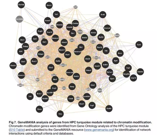
• 这一步就是把选定的模块中的基因导出来，结果包含edges和nodes的信息。导出不同模块的基因只需要改变modules = c("模块颜色名")即可，输出多个模块的信息时，从该行代码运行即可，前面一行的运算量很大。
• edges文件很大，试想一个模块中有500个基因，几乎两两基因之间都有关系，那就有上万条信息，构建出来的网络肯定密密麻麻的用不了。
  这里处理办法有两种：
  1、取Weight值前多少的作用关系；
  2、选定seed基因，比如某个lncRNA或者已知与表型具有密切关联的基因，构建与该基因有关的共表达网络

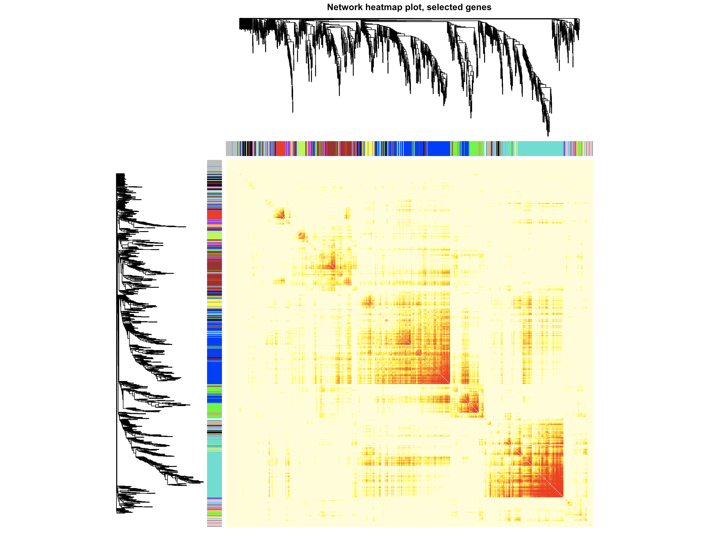
## 可视化基因网络## 
# Calculate topological overlap anew: this could be done more efficiently by saving the TOM
# calculated during module detection, but let us do it again here.
dissTOM = 1-TOMsimilarityFromExpr(datExpr, power = 14);
# Transform dissTOM with a power to make moderately strong connections more visible in the heatmap

plotTOM = dissTOM^7;
# Set diagonal to NA for a nicer plot

diag(plotTOM) = NA;
# Call the plot function#sizeGrWindow(9,9)
TOMplot(plotTOM, geneTree, moduleColors, main = "Network heatmap plot, all genes")
#随便选取1000个基因来可视化
nSelect = 1000
# For reproducibility, we set the random seed
set.seed(10);
select = sample(nGenes, size = nSelect);
selectTOM = dissTOM[select, select];
# There's no simple way of restricting a clustering tree to a subset of genes, so we must re-cluster.
selectTree = hclust(as.dist(selectTOM), method = "average")
selectColors = moduleColors[select];
# Open a graphical window#sizeGrWindow(9,9)
# Taking the dissimilarity to a power, say 10, makes the plot more informative by effectively changing# the color palette; setting the diagonal to NA also improves the clarity of the plot
plotDiss = selectTOM^7;
diag(plotDiss) = NA;
TOMplot(plotDiss, selectTree, selectColors, main = "Network heatmap plot, selected genes")

• 这里是随机选取1000个基因来可视化模块内基因的相关性，你也可以多取一点，不过取太多容易报错，也没有必要。像结果中天青色和蓝色两个模块的共表达聚类结果还是不错的。

#此处画的是根据基因间表达量进行聚类所得到的各模块间的相关性图
MEs = moduleEigengenes(datExpr, moduleColors)$eigengenes
MET = orderMEs(MEs)
sizeGrWindow(7, 6) 
plotEigengeneNetworks(MET, "Eigengene adjacency heatmap", marHeatmap = c(3,4,2,2), plotDendrograms = FALSE, xLabelsAngle = 90)

• 这个是分析共表达模块之间的相关性分析。
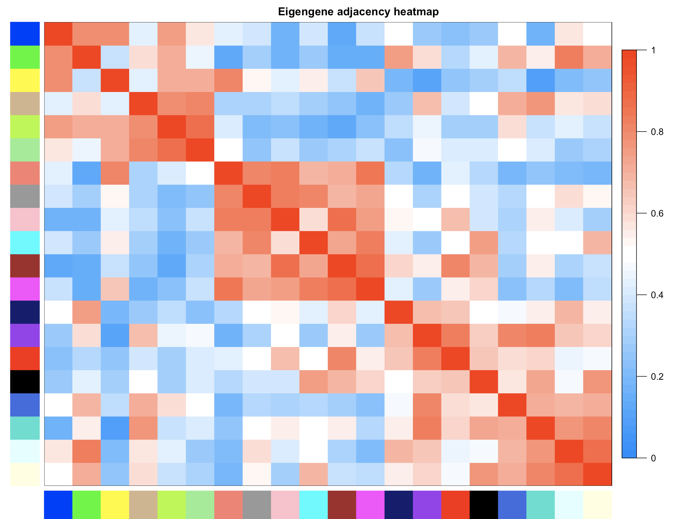
• 到这里，WGCNA的分析基本就结束了。不过，WGCNA分析过程中还有许多其它分析来检验WGCNA分析结果的可信度等等。有兴趣的童鞋可以参看这篇文章：http://www.stat.wisc.edu/~yandell/statgen/ucla/WGCNA/wgcna.html